Session 9: Multivariate Volatility Models
Course: Advanced Volatility Modeling
Learning Objectives
Understand the challenges of multivariate volatility modeling
Implement DCC (Dynamic Conditional Correlation) models
Explore BEKK and other multivariate GARCH specifications
Apply multivariate models to portfolio risk management
1. Multivariate Volatility: Motivation
1.1 Why Multivariate?
Portfolio risk: Need covariances, not just variances
Contagion: Volatility spillovers across assets
Hedging: Dynamic hedge ratios
Time-varying correlations: Correlations increase in crises
1.2 The Curse of Dimensionality
For assets, covariance matrix has unique elements.
| N | Parameters |
|---|---|
| 2 | 3 |
| 10 | 55 |
| 100 | 5,050 |
Need parsimonious specifications!
Source
import numpy as np
import pandas as pd
import matplotlib.pyplot as plt
from scipy.optimize import minimize
from arch import arch_model
import yfinance as yf
import warnings
warnings.filterwarnings('ignore')

plt.style.use('seaborn-v0_8-whitegrid')
plt.rcParams['figure.figsize'] = (12, 6)
np.random.seed(42)
Source
# Download data for multiple assets
tickers = ['SPY', 'EFA', 'TLT', 'GLD']  # US equity, Intl equity, Bonds, Gold
data = yf.download(tickers, start='2010-01-01', end='2024-12-31', progress=False)['Close']

returns = (np.log(data / data.shift(1)) * 100).dropna()
print(f"Assets: {list(returns.columns)}")
print(f"Sample: {returns.index[0].date()} to {returns.index[-1].date()}")
print(f"Observations: {len(returns)}")
YF.download() has changed argument auto_adjust default to True
Assets: ['EFA', 'GLD', 'SPY', 'TLT']
Sample: 2010-01-05 to 2024-12-30
Observations: 3772
Source
# Rolling correlations show time variation
window = 60

fig, axes = plt.subplots(2, 2, figsize=(14, 10))
axes = axes.flatten()

pairs = [('SPY', 'EFA'), ('SPY', 'TLT'), ('SPY', 'GLD'), ('TLT', 'GLD')]

for ax, (a1, a2) in zip(axes, pairs):
    rolling_corr = returns[a1].rolling(window).corr(returns[a2])
    ax.plot(rolling_corr.index, rolling_corr.values, linewidth=0.8)
    ax.axhline(returns[a1].corr(returns[a2]), color='red', linestyle='--',
               label=f'Unconditional: {returns[a1].corr(returns[a2]):.2f}')
    ax.set_title(f'{a1} - {a2}')
    ax.set_ylabel('Correlation')
    ax.legend()
    ax.set_ylim(-1, 1)

plt.suptitle(f'{window}-Day Rolling Correlations', fontsize=14)
plt.tight_layout()
plt.show()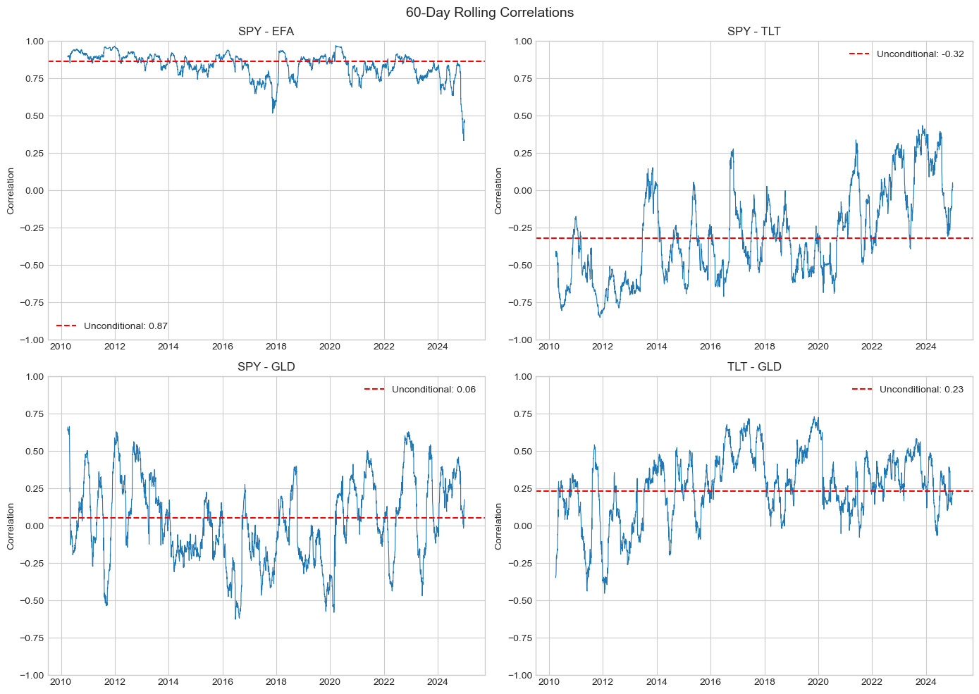
2. DCC Model (Engle, 2002)
2.1 Two-Step Approach
Step 1: Fit univariate GARCH to each series
Step 2: Model correlations of standardized residuals
2.2 DCC Specification
where:
: diagonal matrix of volatilities
: time-varying correlation matrix
Source
def fit_univariate_garch(returns_df):
    """Step 1: Fit GARCH(1,1) to each series."""
    models = {}
    volatilities = pd.DataFrame(index=returns_df.index)
    std_residuals = pd.DataFrame(index=returns_df.index)

    for col in returns_df.columns:
        model = arch_model(returns_df[col], vol='Garch', p=1, q=1)
        fit = model.fit(disp='off')
        models[col] = fit
        volatilities[col] = fit.conditional_volatility
        std_residuals[col] = fit.std_resid

    return models, volatilities, std_residuals.dropna()

# Fit univariate models
garch_models, volatilities, std_resid = fit_univariate_garch(returns)

print("Univariate GARCH Parameters:")
print("="*60)
for col, model in garch_models.items():
    params = model.params
    print(f"\n{col}:")
    print(f"  ω = {params['omega']:.6f}")
    print(f"  α = {params['alpha[1]']:.4f}")
    print(f"  β = {params['beta[1]']:.4f}")
    print(f"  Persistence = {params['alpha[1]'] + params['beta[1]']:.4f}")
Univariate GARCH Parameters:
============================================================
EFA:
ω = 0.025149
α = 0.1256
β = 0.8598
Persistence = 0.9854
GLD:
ω = 0.018372
α = 0.0540
β = 0.9272
Persistence = 0.9813
SPY:
ω = 0.037661
α = 0.1692
β = 0.7987
Persistence = 0.9679
TLT:
ω = 0.016410
α = 0.0670
β = 0.9146
Persistence = 0.9816
Source
def dcc_loglik(params, std_resid):
    """
    DCC log-likelihood (Step 2).

    Parameters
    ----------
    params : array
        [a, b] DCC parameters
    std_resid : DataFrame
        Standardized residuals from Step 1
    """
    a, b = params

    # Constraints
    if a < 0 or b < 0 or a + b >= 1:
        return 1e10

    z = std_resid.values
    T, N = z.shape

    # Unconditional correlation
    Q_bar = np.corrcoef(z.T)

    # Initialize
    Q = Q_bar.copy()
    loglik = 0

    for t in range(T):
        # Update Q
        if t > 0:
            z_tm1 = z[t-1:t].T
            Q = (1 - a - b) * Q_bar + a * (z_tm1 @ z_tm1.T) + b * Q

        # Convert Q to correlation matrix R
        Q_diag_inv_sqrt = np.diag(1 / np.sqrt(np.diag(Q)))
        R = Q_diag_inv_sqrt @ Q @ Q_diag_inv_sqrt

        # Log-likelihood contribution
        try:
            det_R = np.linalg.det(R)
            if det_R <= 0:
                return 1e10
            R_inv = np.linalg.inv(R)
            z_t = z[t:t+1].T
            loglik += -0.5 * (np.log(det_R) + z_t.T @ R_inv @ z_t - z_t.T @ z_t)
        except:
            return 1e10

    return -float(loglik)

def fit_dcc(std_resid):
    """Fit DCC model (Step 2)."""
    result = minimize(
        dcc_loglik,
        [0.05, 0.90],
        args=(std_resid,),
        method='Nelder-Mead',
        options={'maxiter': 1000}
    )
    return result

# Fit DCC
dcc_result = fit_dcc(std_resid)
a_hat, b_hat = dcc_result.x

print("DCC Estimation Results")
print("="*50)
print(f"a = {a_hat:.4f}")
print(f"b = {b_hat:.4f}")
print(f"Persistence (a+b) = {a_hat + b_hat:.4f}")
DCC Estimation Results
==================================================
a = 0.0338
b = 0.9486
Persistence (a+b) = 0.9823
Source
def compute_dcc_correlations(std_resid, a, b):
    """Compute time-varying correlations from DCC model."""
    z = std_resid.values
    T, N = z.shape

    Q_bar = np.corrcoef(z.T)
    Q = Q_bar.copy()

    correlations = np.zeros((T, N, N))

    for t in range(T):
        if t > 0:
            z_tm1 = z[t-1:t].T
            Q = (1 - a - b) * Q_bar + a * (z_tm1 @ z_tm1.T) + b * Q

        Q_diag_inv_sqrt = np.diag(1 / np.sqrt(np.diag(Q)))
        R = Q_diag_inv_sqrt @ Q @ Q_diag_inv_sqrt
        correlations[t] = R

    return correlations

# Compute DCC correlations
dcc_corr = compute_dcc_correlations(std_resid, a_hat, b_hat)

# Plot dynamic correlations
fig, axes = plt.subplots(2, 2, figsize=(14, 10))
axes = axes.flatten()
cols = list(std_resid.columns)

idx_pairs = [(0, 1), (0, 2), (0, 3), (2, 3)]
labels = [f'{cols[i]}-{cols[j]}' for i, j in idx_pairs]

for ax, (i, j), label in zip(axes, idx_pairs, labels):
    dcc_series = dcc_corr[:, i, j]
    ax.plot(std_resid.index, dcc_series, linewidth=0.8, label='DCC')
    ax.axhline(np.corrcoef(std_resid.iloc[:, i], std_resid.iloc[:, j])[0,1],
               color='red', linestyle='--', label='Unconditional')
    ax.set_title(label)
    ax.set_ylabel('Correlation')
    ax.legend()
    ax.set_ylim(-1, 1)

plt.suptitle('DCC Dynamic Correlations', fontsize=14)
plt.tight_layout()
plt.show()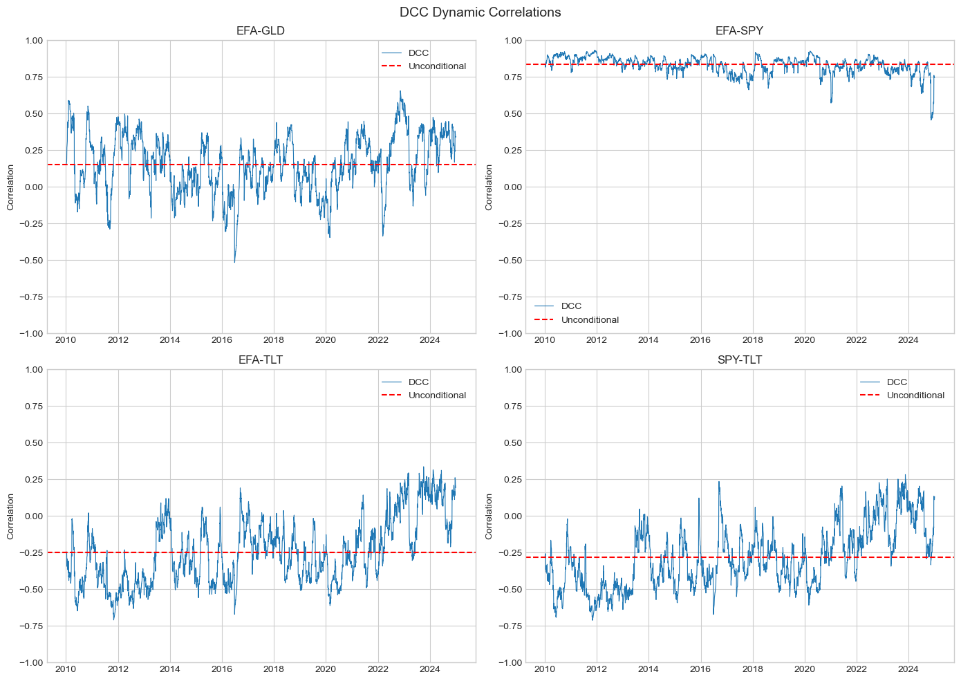
3. BEKK Model
3.1 Specification (Engle & Kroner, 1995)
where (lower triangular), , are matrices.
3.2 Scalar BEKK
For parsimony, assume and :
Source
def scalar_bekk_loglik(params, returns):
    """
    Scalar BEKK log-likelihood.

    H_t = C'C + a² * eps_{t-1} eps_{t-1}' + b² * H_{t-1}
    """
    r = returns.values
    T, N = r.shape

    # Extract parameters
    n_c = N * (N + 1) // 2  # Lower triangular elements
    c_params = params[:n_c]
    a, b = params[n_c], params[n_c + 1]

    # Constraints
    if a < 0 or b < 0 or a**2 + b**2 >= 1:
        return 1e10

    # Build C matrix
    C = np.zeros((N, N))
    idx = 0
    for i in range(N):
        for j in range(i + 1):
            C[i, j] = c_params[idx]
            idx += 1

    CC = C @ C.T

    # Sample covariance for initialization
    H = np.cov(r.T)

    loglik = 0
    for t in range(1, T):
        eps = r[t-1:t].T
        H = CC + a**2 * (eps @ eps.T) + b**2 * H

        try:
            det_H = np.linalg.det(H)
            if det_H <= 0:
                return 1e10
            H_inv = np.linalg.inv(H)
            r_t = r[t:t+1].T
            loglik += -0.5 * (N * np.log(2*np.pi) + np.log(det_H) + r_t.T @ H_inv @ r_t)
        except:
            return 1e10

    return -float(loglik)

# Fit Scalar BEKK (2 assets for speed)
returns_2 = returns[['SPY', 'TLT']]
N = 2
n_c = N * (N + 1) // 2

# Initial values
cov_init = np.cov(returns_2.values.T)
C_init = np.linalg.cholesky(cov_init * 0.1)
c_init = [C_init[i, j] for i in range(N) for j in range(i + 1)]

result_bekk = minimize(
    scalar_bekk_loglik,
    c_init + [0.2, 0.9],
    args=(returns_2,),
    method='Nelder-Mead',
    options={'maxiter': 2000}
)

a_bekk = result_bekk.x[n_c]
b_bekk = result_bekk.x[n_c + 1]

print("Scalar BEKK Results (SPY-TLT)")
print("="*50)
print(f"a = {a_bekk:.4f}")
print(f"b = {b_bekk:.4f}")
print(f"Persistence (a²+b²) = {a_bekk**2 + b_bekk**2:.4f}")
Scalar BEKK Results (SPY-TLT)
==================================================
a = 0.3071
b = 0.9388
Persistence (a²+b²) = 0.9757
4. Portfolio Risk Application
Source
def compute_portfolio_vol(weights, H):
    """Compute portfolio volatility from covariance matrix."""
    w = np.array(weights).reshape(-1, 1)
    return np.sqrt(w.T @ H @ w)[0, 0]

# Compute DCC covariance matrices
def compute_dcc_covariances(volatilities, dcc_corr):
    """Convert DCC correlations to covariances."""
    T = len(volatilities)
    N = volatilities.shape[1]
    H = np.zeros((T, N, N))

    for t in range(T):
        D = np.diag(volatilities.iloc[t].values)
        H[t] = D @ dcc_corr[t] @ D

    return H

# Equal-weight portfolio
weights = np.array([0.25, 0.25, 0.25, 0.25])

# Align volatilities with std_resid index
vol_aligned = volatilities.loc[std_resid.index]
H_dcc = compute_dcc_covariances(vol_aligned, dcc_corr)

# Portfolio volatility over time
port_vol = [compute_portfolio_vol(weights, H_dcc[t]) * np.sqrt(252) for t in range(len(std_resid))]

# Constant correlation benchmark
corr_const = np.corrcoef(returns.T)
vol_mean = volatilities.mean()
D_const = np.diag(vol_mean.values)
H_const = D_const @ corr_const @ D_const
port_vol_const = compute_portfolio_vol(weights, H_const) * np.sqrt(252)

fig, ax = plt.subplots(figsize=(14, 5))
ax.plot(std_resid.index, port_vol, linewidth=0.8, label='DCC Portfolio Vol')
ax.axhline(port_vol_const, color='red', linestyle='--', label=f'Constant Corr Vol: {port_vol_const:.1f}%')
ax.set_ylabel('Annualized Volatility (%)')
ax.set_title('Equal-Weight Portfolio: DCC vs Constant Correlation')
ax.legend()
plt.show()

print(f"\nAverage DCC portfolio vol: {np.mean(port_vol):.2f}%")
print(f"Max DCC portfolio vol: {np.max(port_vol):.2f}%")
print(f"Constant correlation vol: {port_vol_const:.2f}%")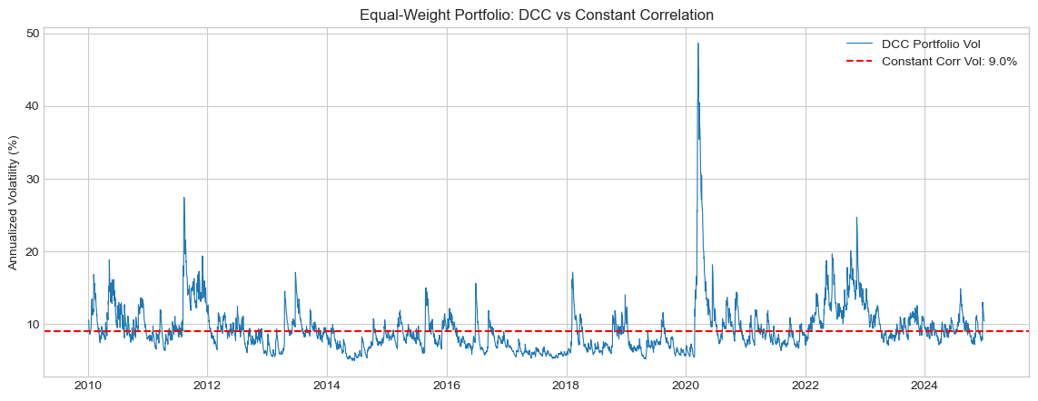
Average DCC portfolio vol: 9.24%
Max DCC portfolio vol: 48.61%
Constant correlation vol: 9.00%
5. Summary
Key Takeaways
DCC: Two-step approach - univariate GARCH then correlation dynamics
BEKK: Direct modeling of covariance matrix (more parameters)
Time-varying correlations: Crucial for risk management
Portfolio risk: DCC captures crisis correlation spikes
Preview: Session 10
Path-dependent volatility and practical applications.
Exercises
Implement asymmetric DCC (ADCC) with leverage effect
Compare DCC vs rolling correlation for hedge ratios
Estimate DCC for crypto-equity portfolio
Backtest minimum variance portfolio with DCC vs constant correlation
References
Engle, R. (2002). Dynamic conditional correlation. Journal of Business & Economic Statistics, 20(3), 339-350.
Engle, R. F., & Kroner, K. F. (1995). Multivariate simultaneous generalized ARCH. Econometric Theory, 11(1), 122-150.
Bauwens, L., Laurent, S., & Rombouts, J. V. (2006). Multivariate GARCH models: a survey. Journal of Applied Econometrics, 21(1), 79-109.