Session 10: Path-Dependent Volatility and Applications
Course: Advanced Volatility Modeling
Learning Objectives
Understand path-dependent volatility dynamics
Implement volatility targeting and risk parity strategies
Apply volatility models to VaR and Expected Shortfall
Explore volatility in option pricing and the VIX
1. Path-Dependent Volatility
1.1 What is Path Dependence?
Volatility depends not just on the current state but on the path of past returns:
GARCH: depends on
HAR: Uses daily, weekly, monthly averages of RV
Regime switching: Volatility depends on current regime and transition history
1.2 Signature of Path Dependence
At-the-money implied volatility responds to:
Recent realized volatility
Recent returns (leverage effect)
Time since last volatility spike
Source
import numpy as np
import pandas as pd
import matplotlib.pyplot as plt
from scipy import stats
from arch import arch_model
import yfinance as yf
import warnings
warnings.filterwarnings('ignore')

plt.style.use('seaborn-v0_8-whitegrid')
plt.rcParams['figure.figsize'] = (12, 6)
np.random.seed(42)
Source
# Download data
spy = yf.download('SPY', start='2010-01-01', end='2024-12-31', progress=False)
vix = yf.download('^VIX', start='2010-01-01', end='2024-12-31', progress=False)

if isinstance(spy.columns, pd.MultiIndex):
    spy.columns = spy.columns.get_level_values(0)
    vix.columns = vix.columns.get_level_values(0)

data = pd.DataFrame({
    'price': spy['Close'],
    'vix': vix['Close']
}).dropna()

data['returns'] = np.log(data['price'] / data['price'].shift(1)) * 100
data['rv_20'] = data['returns'].rolling(20).std() * np.sqrt(252)  # Annualized
data = data.dropna()

print(f"Sample: {data.index[0].date()} to {data.index[-1].date()}")
YF.download() has changed argument auto_adjust default to True
Sample: 2010-02-02 to 2024-12-30
2. Volatility Targeting
2.1 Concept
Adjust portfolio exposure inversely to volatility:
where is the target volatility.
2.2 Benefits
Constant risk contribution
Reduced drawdowns during crises
More stable Sharpe ratio
Source
def volatility_targeting_strategy(returns, vol_forecast, target_vol=10, max_leverage=2):
    """
    Implement volatility targeting strategy.

    Parameters
    ----------
    returns : Series
        Asset returns
    vol_forecast : Series
        Volatility forecast (annualized %)
    target_vol : float
        Target volatility (%)
    max_leverage : float
        Maximum leverage allowed
    """
    # Compute weights
    weights = target_vol / vol_forecast
    weights = weights.clip(0, max_leverage)  # Cap leverage

    # Lag weights by 1 day (use yesterday's forecast for today's position)
    weights = weights.shift(1)

    # Strategy returns
    strat_returns = weights * returns

    return strat_returns, weights

# Fit GARCH for volatility forecast
garch = arch_model(data['returns'], vol='Garch', p=1, q=1)
garch_fit = garch.fit(disp='off')
vol_forecast = garch_fit.conditional_volatility * np.sqrt(252)  # Annualize

# Run strategy
target_vol = 10  # 10% target
strat_returns, weights = volatility_targeting_strategy(
    data['returns'], vol_forecast, target_vol=target_vol
)

# Compare
results = pd.DataFrame({
    'Buy & Hold': data['returns'],
    'Vol Target': strat_returns,
    'Weight': weights
}).dropna()

# Cumulative returns
cum_bh = (1 + results['Buy & Hold']/100).cumprod()
cum_vt = (1 + results['Vol Target']/100).cumprod()

fig, axes = plt.subplots(3, 1, figsize=(14, 12))

axes[0].plot(cum_bh.index, cum_bh, label='Buy & Hold', linewidth=1)
axes[0].plot(cum_vt.index, cum_vt, label='Vol Target', linewidth=1)
axes[0].set_ylabel('Cumulative Return')
axes[0].set_title('Volatility Targeting Strategy')
axes[0].legend()
axes[0].set_yscale('log')

axes[1].plot(results['Weight'].index, results['Weight'], linewidth=0.8)
axes[1].axhline(1, color='red', linestyle='--')
axes[1].set_ylabel('Leverage')
axes[1].set_title('Dynamic Leverage')

axes[2].plot(vol_forecast.index, vol_forecast, label='GARCH Forecast', linewidth=0.8)
axes[2].axhline(target_vol, color='red', linestyle='--', label=f'Target: {target_vol}%')
axes[2].set_ylabel('Volatility (%)')
axes[2].set_title('Volatility Forecast')
axes[2].legend()

plt.tight_layout()
plt.show()

# Performance metrics
def performance_metrics(returns):
    ann_ret = returns.mean() * 252
    ann_vol = returns.std() * np.sqrt(252)
    sharpe = ann_ret / ann_vol
    max_dd = (returns.cumsum() - returns.cumsum().cummax()).min()
    return ann_ret, ann_vol, sharpe, max_dd

print("\nPerformance Comparison")
print("="*60)
print(f"{'Metric':<20} {'Buy & Hold':>15} {'Vol Target':>15}")
print("-"*60)

bh_metrics = performance_metrics(results['Buy & Hold'])
vt_metrics = performance_metrics(results['Vol Target'])

for metric, bh, vt in zip(['Ann. Return (%)', 'Ann. Volatility (%)', 'Sharpe Ratio', 'Max Drawdown (%)'],
                          bh_metrics, vt_metrics):
    print(f"{metric:<20} {bh:>15.2f} {vt:>15.2f}")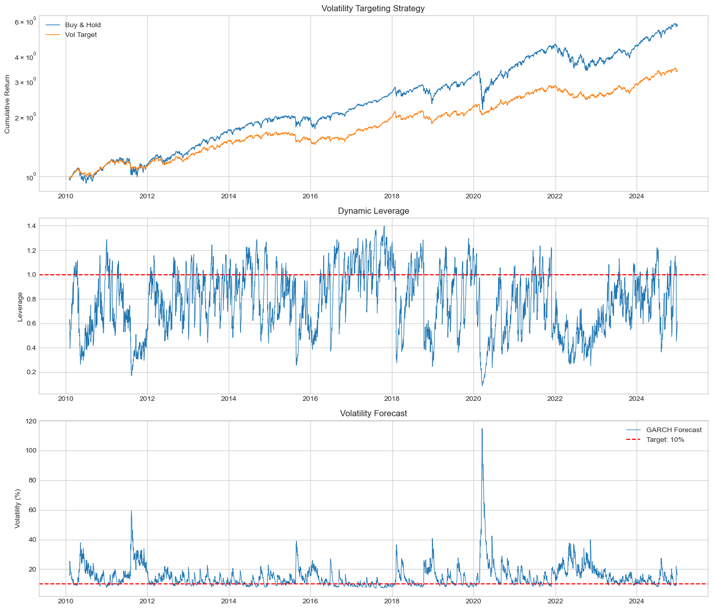
Performance Comparison
============================================================
Metric                    Buy & Hold      Vol Target
------------------------------------------------------------
Ann. Return (%)                13.09            8.63
Ann. Volatility (%)            17.10           10.09
Sharpe Ratio                    0.77            0.85
Max Drawdown (%)              -41.12          -15.53
3. Value at Risk (VaR) and Expected Shortfall
3.1 Definitions
Value at Risk at confidence level :
Expected Shortfall (Conditional VaR):
Source
def garch_var_es(returns, alpha=0.01, window=500):
    """
    Compute rolling VaR and ES using GARCH.
    """
    n = len(returns)
    var_list = []
    es_list = []
    dates = []

    for t in range(window, n):
        train = returns.iloc[t-window:t]

        try:
            model = arch_model(train, vol='Garch', p=1, q=1, dist='t')
            fit = model.fit(disp='off', show_warning=False)

            # 1-day forecast
            forecast = fit.forecast(horizon=1, reindex=False)
            vol_forecast = np.sqrt(forecast.variance.iloc[-1, 0])

            # Degrees of freedom
            nu = fit.params.get('nu', 8)

            # VaR (Student-t)
            var_t = -stats.t.ppf(alpha, nu) * vol_forecast * np.sqrt((nu-2)/nu)

            # ES (Student-t)
            t_alpha = stats.t.ppf(alpha, nu)
            es_t = vol_forecast * np.sqrt((nu-2)/nu) * (
                stats.t.pdf(t_alpha, nu) / alpha * (nu + t_alpha**2) / (nu - 1)
            )

            var_list.append(var_t)
            es_list.append(es_t)
            dates.append(returns.index[t])
        except:
            continue

    return pd.DataFrame({'VaR': var_list, 'ES': es_list}, index=dates)

# Compute rolling VaR/ES
risk_measures = garch_var_es(data['returns'], alpha=0.01, window=500)

# Align returns
returns_aligned = data['returns'].loc[risk_measures.index]

# Count violations
violations = (returns_aligned < -risk_measures['VaR']).sum()
violation_rate = violations / len(risk_measures) * 100

print(f"VaR Backtest (1% level)")
print(f"="*40)
print(f"Expected violations: 1.00%")
print(f"Actual violations: {violation_rate:.2f}%")
print(f"Number of violations: {violations} / {len(risk_measures)}")
VaR Backtest (1% level)
========================================
Expected violations: 1.00%
Actual violations: 1.44%
Number of violations: 47 / 3253
Source
# Plot VaR backtest
fig, ax = plt.subplots(figsize=(14, 6))

ax.plot(returns_aligned.index, returns_aligned, 'b-', linewidth=0.5, alpha=0.6, label='Returns')
ax.plot(risk_measures.index, -risk_measures['VaR'], 'r-', linewidth=1, label='1% VaR')
ax.plot(risk_measures.index, -risk_measures['ES'], 'g--', linewidth=1, label='1% ES')

# Mark violations
violations_mask = returns_aligned < -risk_measures['VaR']
ax.scatter(returns_aligned[violations_mask].index,
           returns_aligned[violations_mask],
           color='red', s=20, zorder=5, label='Violations')

ax.set_ylabel('Returns (%)')
ax.set_title('GARCH VaR Backtest (1% level)')
ax.legend(loc='lower left')

plt.tight_layout()
plt.show()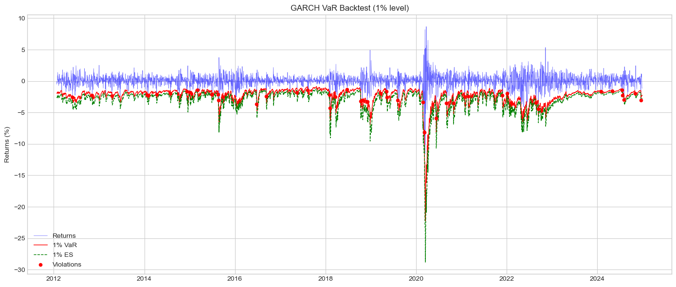
4. VIX and Implied Volatility
4.1 VIX Index
The VIX measures 30-day implied volatility from S&P 500 options:
4.2 VIX-Realized Volatility Spread
The Variance Risk Premium (VRP):
On average, VRP > 0: Investors pay a premium for volatility protection.
Source
# VIX vs Realized Volatility
data['rv_30_fwd'] = data['returns'].rolling(22).std().shift(-22) * np.sqrt(252)

fig, axes = plt.subplots(2, 1, figsize=(14, 10))

# Time series
axes[0].plot(data.index, data['vix'], label='VIX (Implied)', linewidth=0.8)
axes[0].plot(data.index, data['rv_20'], label='20-day Realized Vol', linewidth=0.8, alpha=0.7)
axes[0].set_ylabel('Volatility (%)')
axes[0].set_title('VIX vs Realized Volatility')
axes[0].legend()

# Variance Risk Premium
vrp = data['vix'] - data['rv_20']
axes[1].plot(vrp.index, vrp, linewidth=0.8, color='purple')
axes[1].axhline(vrp.mean(), color='red', linestyle='--', label=f'Mean: {vrp.mean():.1f}')
axes[1].axhline(0, color='black', linewidth=0.5)
axes[1].fill_between(vrp.index, 0, vrp, where=vrp>0, alpha=0.3, color='green')
axes[1].fill_between(vrp.index, 0, vrp, where=vrp<0, alpha=0.3, color='red')
axes[1].set_ylabel('VIX - RV (%)')
axes[1].set_title('Variance Risk Premium')
axes[1].legend()

plt.tight_layout()
plt.show()

print(f"\nVariance Risk Premium Statistics:")
print(f"Mean: {vrp.mean():.2f}%")
print(f"% Positive: {(vrp > 0).mean()*100:.1f}%")
print(f"\nOn average, VIX exceeds realized vol by {vrp.mean():.1f} percentage points.")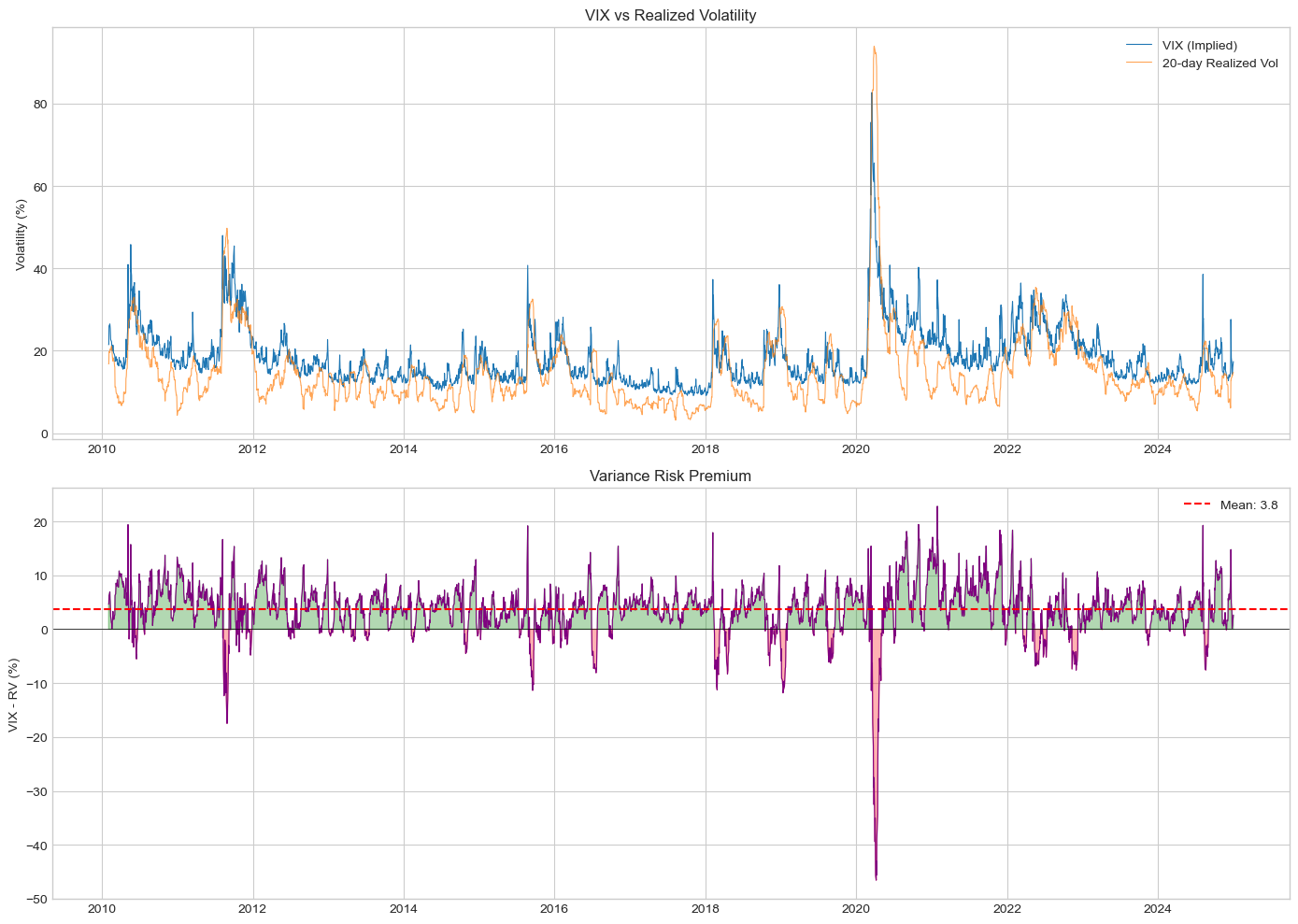
Variance Risk Premium Statistics:
Mean: 3.76%
% Positive: 85.3%

On average, VIX exceeds realized vol by 3.8 percentage points.
5. Volatility Trading Strategies
5.1 Sell Volatility (Variance Swap)
Profit from VRP by selling variance:
Short VIX futures / options
Short variance swaps
Short straddles
Source
# Simple variance selling strategy (conceptual)
# P&L ≈ VIX² - RV² (for variance swap)

data['vix_lag'] = data['vix'].shift(22)  # Entry VIX
data['variance_swap_pnl'] = (data['vix_lag']**2 - data['rv_20']**2) / 100  # Scaled

var_swap_returns = data['variance_swap_pnl'].dropna()

fig, axes = plt.subplots(2, 1, figsize=(14, 8))

# Cumulative P&L
axes[0].plot(var_swap_returns.index, var_swap_returns.cumsum(), linewidth=1)
axes[0].set_ylabel('Cumulative P&L')
axes[0].set_title('Variance Swap Selling Strategy (Conceptual)')

# Monthly returns
monthly_pnl = var_swap_returns.resample('M').sum()
axes[1].bar(monthly_pnl.index, monthly_pnl.values, width=20,
            color=['green' if x > 0 else 'red' for x in monthly_pnl.values])
axes[1].set_ylabel('Monthly P&L')
axes[1].set_title('Monthly Returns')

plt.tight_layout()
plt.show()

print("\nVariance Selling Strategy:")
print(f"Win rate: {(var_swap_returns > 0).mean()*100:.1f}%")
print(f"Average daily P&L: {var_swap_returns.mean():.4f}")
print(f"Sharpe ratio: {var_swap_returns.mean() / var_swap_returns.std() * np.sqrt(252):.2f}")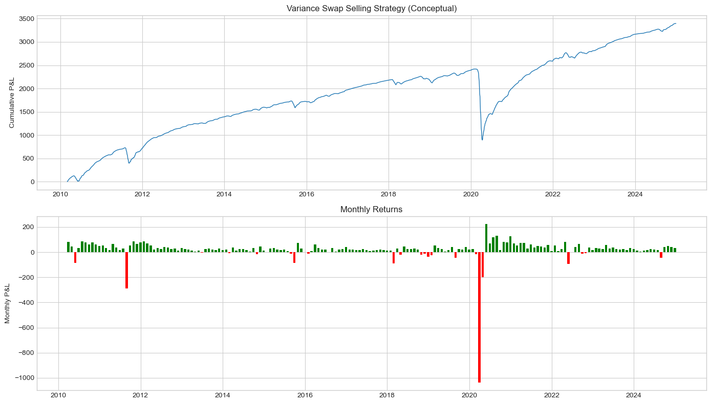
Variance Selling Strategy:
Win rate: 82.8%
Average daily P&L: 0.9099
Sharpe ratio: 2.43
6. Course Summary
Key Models Covered
| Session | Topic | Key Models |
|---|---|---|
| 1 | Foundations | Stylized facts, simple estimators |
| 2 | GARCH | ARCH, GARCH, IGARCH |
| 3 | Asymmetric | GJR-GARCH, EGARCH, TGARCH |
| 4 | Advanced | FIGARCH, APARCH, Component |
| 5 | Realized | RV, BV, TSRV, Realized Kernel |
| 6 | HAR | HAR-RV, HAR-CJ, HAR-RS |
| 7 | Stochastic | SV, Heston |
| 8 | Rough | fBM, Rough Bergomi |
| 9 | Multivariate | DCC, BEKK |
| 10 | Applications | Vol targeting, VaR, VRP |
Final Exercises
Comprehensive Project: Build a complete volatility forecasting system that:
Compares GARCH, HAR, and rough volatility models
Evaluates forecasts using multiple metrics
Applies to portfolio risk management
Cryptocurrency Volatility: Apply all course methods to Bitcoin/Ethereum and document differences from equities
Option Pricing: Implement and compare option prices from Heston vs rough Bergomi
VIX Trading: Design and backtest a VIX-based trading strategy using HAR forecasts
Multivariate Risk: Build a DCC-based risk system for a multi-asset portfolio
References (Course-Wide)
Textbooks
Tsay, R. S. (2010). Analysis of Financial Time Series. Wiley.
Francq, C., & Zakoian, J. M. (2019). GARCH Models. Wiley.
Gatheral, J. (2006). The Volatility Surface. Wiley.
Key Papers
Bollerslev (1986) - GARCH
Nelson (1991) - EGARCH
Engle (2002) - DCC
Corsi (2009) - HAR
Gatheral et al. (2018) - Rough Volatility
Software
Python:
arch,statsmodels,scipyR:
rugarch,rmgarch