Session 7: Stochastic Volatility Models
Course: Advanced Volatility Modeling
Learning Objectives
Understand stochastic volatility (SV) in continuous and discrete time
Compare SV to GARCH: key differences and implications
Estimate SV models using quasi-maximum likelihood
Explore the Heston model and affine structures
1. Stochastic Volatility: Core Idea
1.1 GARCH vs SV
GARCH: Volatility is deterministic given past returns:
Stochastic Volatility: Volatility has its own source of randomness:
where is a shock independent of the return innovation.
1.2 Why Stochastic Volatility?
More realistic: Volatility can change even without large returns
Option pricing: Better fits option smile/skew
Continuous-time foundation: Natural extension of diffusions
Separate risk factors: Volatility risk can be priced separately
Source
import numpy as np
import pandas as pd
import matplotlib.pyplot as plt
from scipy.optimize import minimize
from scipy import stats
import warnings
warnings.filterwarnings('ignore')

plt.style.use('seaborn-v0_8-whitegrid')
plt.rcParams['figure.figsize'] = (12, 6)
np.random.seed(42)
2. Discrete-Time SV Model
2.1 Basic Specification (Taylor, 1986)
where are returns and is log-volatility.
Parameters:
: long-run mean of log-volatility
: persistence (should be < 1 for stationarity)
: volatility of volatility
Source
def simulate_sv(n, mu, phi, sigma_eta, seed=None):
    """
    Simulate discrete-time stochastic volatility model.

    y_t = exp(h_t/2) * eps_t
    h_t = mu + phi*(h_{t-1} - mu) + sigma_eta * eta_t
    """
    if seed is not None:
        np.random.seed(seed)

    h = np.zeros(n)
    y = np.zeros(n)

    eps = np.random.standard_normal(n)
    eta = np.random.standard_normal(n)

    # Initialize at unconditional mean
    h[0] = mu + sigma_eta * eta[0] / np.sqrt(1 - phi**2)
    y[0] = np.exp(h[0] / 2) * eps[0]

    for t in range(1, n):
        h[t] = mu + phi * (h[t-1] - mu) + sigma_eta * eta[t]
        y[t] = np.exp(h[t] / 2) * eps[t]

    return y, h

# Simulate SV process
n = 2500
mu = -10  # exp(-10/2) ≈ 0.0067 daily vol
phi = 0.97
sigma_eta = 0.15

y_sv, h_sv = simulate_sv(n, mu, phi, sigma_eta, seed=42)

# Also simulate GARCH for comparison
def simulate_garch(n, omega, alpha, beta, seed=None):
    if seed is not None:
        np.random.seed(seed)

    eps = np.random.standard_normal(n)
    y = np.zeros(n)
    sigma2 = np.zeros(n)

    sigma2[0] = omega / (1 - alpha - beta)
    y[0] = np.sqrt(sigma2[0]) * eps[0]

    for t in range(1, n):
        sigma2[t] = omega + alpha * y[t-1]**2 + beta * sigma2[t-1]
        y[t] = np.sqrt(sigma2[t]) * eps[t]

    return y, sigma2

y_garch, sigma2_garch = simulate_garch(n, 0.01, 0.05, 0.90, seed=42)

# Compare
fig, axes = plt.subplots(2, 2, figsize=(14, 8))

axes[0,0].plot(y_sv, linewidth=0.5, color='steelblue')
axes[0,0].set_title('Stochastic Volatility: Returns')

axes[0,1].plot(y_garch, linewidth=0.5, color='steelblue')
axes[0,1].set_title('GARCH: Returns')

axes[1,0].plot(np.exp(h_sv/2), linewidth=0.8, color='red')
axes[1,0].set_title('SV: Volatility σ_t')

axes[1,1].plot(np.sqrt(sigma2_garch), linewidth=0.8, color='red')
axes[1,1].set_title('GARCH: Volatility σ_t')

plt.tight_layout()
plt.show()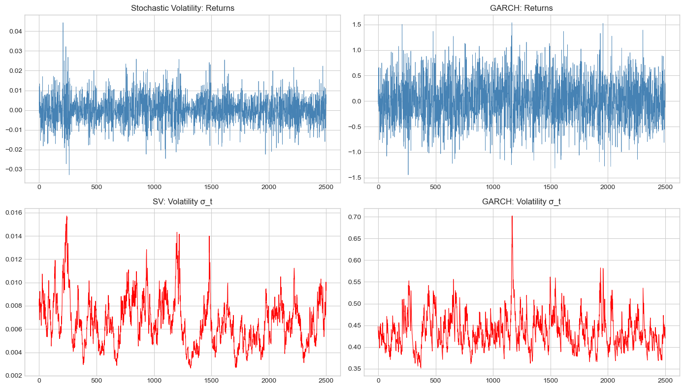
3. Estimation: Quasi-Maximum Likelihood
3.1 The Estimation Challenge
SV models have a non-linear latent state , making exact MLE intractable.
3.2 Harvey et al. (1994) Approach
Transform to linear state-space form by squaring and taking logs:
where with mean -1.27 and variance .
This gives a linear Gaussian state-space model (approximately), enabling Kalman filter estimation.
Source
def sv_qml_loglik(params, y_squared_log):
    """
    Quasi-MLE for SV model using Kalman filter.

    Observation: y*_t = h_t + xi_t, where xi_t ~ log(chi^2_1)
    State: h_t = mu + phi*(h_{t-1} - mu) + sigma_eta * eta_t
    """
    mu, phi, sigma_eta = params

    # Constraints
    if sigma_eta <= 0 or abs(phi) >= 1:
        return 1e10

    T = len(y_squared_log)

    # Constants for log(chi^2_1)
    xi_mean = -1.2704  # E[log(chi^2_1)]
    xi_var = 4.93      # Var[log(chi^2_1)] ≈ pi^2/2

    # Adjust observations
    y_adj = y_squared_log - xi_mean

    # Initialize Kalman filter
    h_pred = mu
    P_pred = sigma_eta**2 / (1 - phi**2)

    loglik = 0

    for t in range(T):
        # Prediction error
        v = y_adj[t] - h_pred
        F = P_pred + xi_var

        # Log-likelihood contribution
        loglik += -0.5 * (np.log(2*np.pi) + np.log(F) + v**2/F)

        # Kalman gain
        K = P_pred / F

        # Update
        h_filt = h_pred + K * v
        P_filt = P_pred * (1 - K)

        # Predict
        h_pred = mu + phi * (h_filt - mu)
        P_pred = phi**2 * P_filt + sigma_eta**2

    return -loglik  # Return negative for minimization

def fit_sv_qml(returns):
    """Fit SV model using QML."""
    # Transform data
    y_sq = returns**2
    y_sq[y_sq == 0] = 1e-10  # Avoid log(0)
    y_log = np.log(y_sq)

    # Initial values
    mu0 = np.mean(y_log)
    phi0 = 0.95
    sigma_eta0 = 0.2

    result = minimize(
        sv_qml_loglik,
        [mu0, phi0, sigma_eta0],
        args=(y_log,),
        method='Nelder-Mead',
        options={'maxiter': 5000}
    )

    return result

# Fit to simulated data
sv_fit = fit_sv_qml(y_sv)

print("Stochastic Volatility QML Estimation")
print("="*50)
print(f"\nTrue parameters:")
print(f"  μ = {mu}")
print(f"  φ = {phi}")
print(f"  σ_η = {sigma_eta}")
print(f"\nEstimated parameters:")
print(f"  μ = {sv_fit.x[0]:.4f}")
print(f"  φ = {sv_fit.x[1]:.4f}")
print(f"  σ_η = {sv_fit.x[2]:.4f}")
Stochastic Volatility QML Estimation
==================================================
True parameters:
μ = -10
φ = 0.97
σ_η = 0.15
Estimated parameters:
μ = -10.1676
φ = 0.9508
σ_η = 0.2196
4. Continuous-Time SV: The Heston Model
4.1 Model Specification
with .
Parameters:
: mean reversion speed
: long-run variance
: volatility of volatility
: leverage correlation (typically negative)
4.2 Feller Condition
ensures variance stays positive.
Source
def simulate_heston(T, n_steps, S0, V0, mu, kappa, theta, sigma_v, rho, seed=None):
"""
Simulate Heston stochastic volatility model using Euler discretization.
"""
if seed is not None:
np.random.seed(seed)
dt = T / n_steps
S = np.zeros(n_steps + 1)
V = np.zeros(n_steps + 1)
S[0] = S0
V[0] = V0
for i in range(n_steps):
# Correlated Brownian motions
Z1 = np.random.standard_normal()
Z2 = np.random.standard_normal()
W_S = Z1
W_V = rho * Z1 + np.sqrt(1 - rho**2) * Z2
# Ensure variance stays positive (full truncation)
V_pos = max(V[i], 0)
# Euler step
S[i+1] = S[i] * np.exp((mu - 0.5*V_pos)*dt + np.sqrt(V_pos*dt)*W_S)
V[i+1] = V[i] + kappa*(theta - V_pos)*dt + sigma_v*np.sqrt(V_pos*dt)*W_V
V[i+1] = max(V[i+1], 0) # Reflection
return S, V
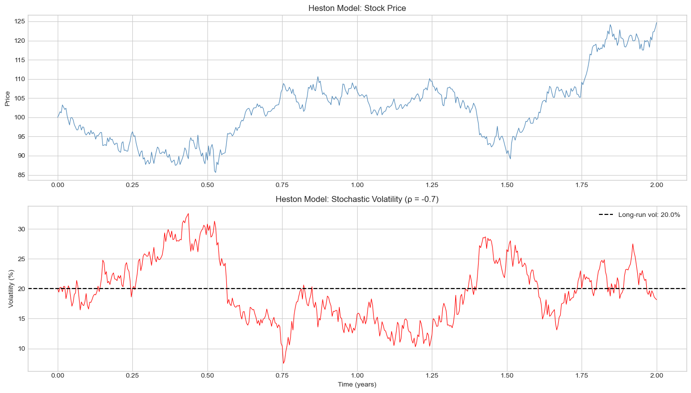
# Simulate Heston model
T = 2 # years
n_steps = 252 * 2 # daily
S0, V0 = 100, 0.04 # Initial price and variance
mu = 0.05
kappa = 3.0
theta = 0.04
sigma_v = 0.4
rho = -0.7
# Check Feller condition
feller = 2 * kappa * theta
print(f"Feller condition: 2κθ = {feller:.4f} vs σ²_v = {sigma_v**2:.4f}")
print(f"Condition {'satisfied' if feller > sigma_v**2 else 'VIOLATED'}")
S_heston, V_heston = simulate_heston(T, n_steps, S0, V0, mu, kappa, theta, sigma_v, rho, seed=42)
# Plot
fig, axes = plt.subplots(2, 1, figsize=(14, 8))
t = np.linspace(0, T, n_steps + 1)
axes[0].plot(t, S_heston, color='steelblue', linewidth=0.8)
axes[0].set_ylabel('Price')
axes[0].set_title('Heston Model: Stock Price', fontsize=12)
axes[1].plot(t, np.sqrt(V_heston) * 100, color='red', linewidth=0.8)
axes[1].axhline(np.sqrt(theta) * 100, color='black', linestyle='--',
label=f'Long-run vol: {np.sqrt(theta)*100:.1f}%')
axes[1].set_xlabel('Time (years)')
axes[1].set_ylabel('Volatility (%)')
axes[1].set_title(f'Heston Model: Stochastic Volatility (ρ = {rho})', fontsize=12)
axes[1].legend()
plt.tight_layout()
plt.show()Feller condition: 2κθ = 0.2400 vs σ²_v = 0.1600
Condition satisfied
5. SV with Leverage
5.1 Correlated Innovations
In discrete time, introduce correlation:
Negative captures the leverage effect: negative returns → higher volatility.
Source
def simulate_sv_leverage(n, mu, phi, sigma_eta, rho, seed=None):
    """SV model with leverage (correlated innovations)."""
    if seed is not None:
        np.random.seed(seed)

    h = np.zeros(n)
    y = np.zeros(n)

    # Correlated innovations
    for t in range(n):
        z1 = np.random.standard_normal()
        z2 = np.random.standard_normal()

        eps = z1
        eta = rho * z1 + np.sqrt(1 - rho**2) * z2

        if t == 0:
            h[t] = mu + sigma_eta * eta / np.sqrt(1 - phi**2)
        else:
            h[t] = mu + phi * (h[t-1] - mu) + sigma_eta * eta

        y[t] = np.exp(h[t] / 2) * eps

    return y, h

# Compare with and without leverage
n = 2000
mu, phi, sigma_eta = -10, 0.97, 0.15

y_no_lev, h_no_lev = simulate_sv(n, mu, phi, sigma_eta, seed=42)
y_lev, h_lev = simulate_sv_leverage(n, mu, phi, sigma_eta, rho=-0.5, seed=42)

# Compute correlation of returns with future volatility change
def leverage_correlation(y, h, lag=1):
    dh = np.diff(h[lag:])
    r = y[:-lag-1]
    return np.corrcoef(r, dh)[0, 1]

print("Leverage Effect in SV Models")
print("="*50)
print(f"Corr(r_t, Δh_{{t+1}}) without leverage: {leverage_correlation(y_no_lev, h_no_lev):.4f}")
print(f"Corr(r_t, Δh_{{t+1}}) with leverage (ρ=-0.5): {leverage_correlation(y_lev, h_lev):.4f}")
Leverage Effect in SV Models
==================================================
Corr(r_t, Δh_{t+1}) without leverage: 0.0172
Corr(r_t, Δh_{t+1}) with leverage (ρ=-0.5): 0.0326
6. Comparison: SV vs GARCH
| Feature | GARCH | Stochastic Volatility |
|---|---|---|
| Volatility dynamics | Deterministic given past | Random (own shock) |
| Estimation | MLE (straightforward) | Challenging (latent state) |
| Option pricing | Requires simulation | Closed-form (Heston) |
| Leverage | GJR-GARCH | Correlated innovations |
| Kurtosis | From GARCH dynamics | Can be more flexible |
7. Summary
Key Takeaways
Stochastic Volatility has separate randomness for volatility
Heston model is the workhorse continuous-time SV model
QML estimation via log-squared returns transformation
Leverage captured by correlation between return and volatility innovations
Preview: Session 8
Rough volatility - fractional Brownian motion in volatility.
Exercises
Implement the MCMC (Markov Chain Monte Carlo) estimator for SV
Simulate Heston paths and price a European call option
Compare volatility forecasts from GARCH vs SV
Estimate SV model with leverage on S&P 500 returns
References
Taylor, S. J. (1986). Modelling Financial Time Series. Wiley.
Harvey, A., Ruiz, E., & Shephard, N. (1994). Multivariate stochastic variance models. Review of Economic Studies, 61(2), 247-264.
Heston, S. L. (1993). A closed-form solution for options with stochastic volatility. Review of Financial Studies, 6(2), 327-343.