Session 6: HAR Models and Realized Measures
Course: Advanced Volatility Modeling
Learning Objectives
Understand the Heterogeneous Autoregressive (HAR) model
Implement HAR-RV and extensions (HAR-RV-J, HAR-RV-CJ)
Forecast realized volatility and evaluate forecast performance
Work with realized semivariance and signed measures
1. The HAR Model
1.1 Motivation: Heterogeneous Market Hypothesis
Müller et al. (1997) proposed that markets contain agents operating at different time horizons:
Daily traders: react to daily information
Weekly traders: institutional investors, portfolio rebalancing
Monthly traders: long-term investors, pension funds
1.2 HAR-RV Model (Corsi, 2009)
where:
: daily RV
: weekly average
: monthly average
1.3 Key Properties
Simple linear model (OLS estimation)
Captures long memory through cascade of components
Often outperforms GARCH for RV forecasting
Source
import numpy as np
import pandas as pd
import matplotlib.pyplot as plt
import statsmodels.api as sm
from scipy import stats
import yfinance as yf
import warnings
warnings.filterwarnings('ignore')

plt.style.use('seaborn-v0_8-whitegrid')
plt.rcParams['figure.figsize'] = (12, 6)
np.random.seed(42)
Source
def simulate_rv_series(n_days, omega=0.1, d_coef=0.3, persistence=0.97):
    """Simulate daily RV series with long memory."""
    rv = np.zeros(n_days)
    rv[0] = omega / (1 - persistence)

    for t in range(1, n_days):
        shock = np.random.exponential(1) - 1
        rv[t] = omega + persistence * rv[t-1] + d_coef * shock * np.sqrt(rv[t-1])
        rv[t] = max(rv[t], 0.01)

    return rv

# Simulate RV series
n_days = 3000
rv_sim = simulate_rv_series(n_days)
dates = pd.date_range('2012-01-01', periods=n_days, freq='B')
rv_series = pd.Series(rv_sim, index=dates, name='RV')

fig, ax = plt.subplots(figsize=(14, 5))
ax.plot(rv_series.index, np.sqrt(rv_series) * np.sqrt(252) * 100, linewidth=0.8)
ax.set_ylabel('Annualized Volatility (%)')
ax.set_title('Simulated Daily Realized Volatility')
plt.show()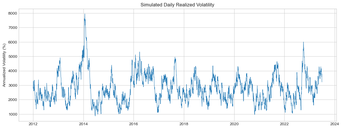
Source
def prepare_har_data(rv, horizon=1):
    """
    Prepare data for HAR model estimation.

    Parameters
    ----------
    rv : pd.Series
        Daily realized variance
    horizon : int
        Forecast horizon in days

    Returns
    -------
    DataFrame with y and X variables
    """
    df = pd.DataFrame(index=rv.index)

    # Target: h-day ahead RV (or average for h>1)
    if horizon == 1:
        df['y'] = rv.shift(-1)
    else:
        df['y'] = rv.rolling(horizon).mean().shift(-horizon)

    # Regressors (lagged)
    df['RV_d'] = rv  # Daily
    df['RV_w'] = rv.rolling(5).mean()  # Weekly
    df['RV_m'] = rv.rolling(22).mean()  # Monthly

    return df.dropna()

def fit_har(rv, horizon=1):
    """Estimate HAR-RV model."""
    df = prepare_har_data(rv, horizon)

    y = df['y']
    X = sm.add_constant(df[['RV_d', 'RV_w', 'RV_m']])

    model = sm.OLS(y, X).fit(cov_type='HAC', cov_kwds={'maxlags': 5})
    return model, df

# Fit HAR model
har_model, har_data = fit_har(rv_series, horizon=1)

print("HAR-RV Model Estimation")
print("="*60)
print(har_model.summary().tables[1])

print(f"\nR² = {har_model.rsquared:.4f}")
print(f"Adj. R² = {har_model.rsquared_adj:.4f}")
HAR-RV Model Estimation
============================================================
==============================================================================
coef std err z P>|z| [0.025 0.975]
------------------------------------------------------------------------------
const 0.0831 0.025 3.286 0.001 0.034 0.133
RV_d 1.0191 0.036 28.384 0.000 0.949 1.089
RV_w -0.0500 0.038 -1.316 0.188 -0.124 0.024
RV_m 0.0071 0.013 0.534 0.593 -0.019 0.033
==============================================================================
R² = 0.9546
Adj. R² = 0.9546
2. HAR Extensions
2.1 HAR-RV-J: Adding Jump Component
where .
2.2 HAR-RV-CJ: Continuous and Jump Components
where (continuous component).
Source
def simulate_rv_with_jumps(n_days, base_vol=0.15, jump_prob=0.05, jump_size=0.5):
    """Simulate RV series with separate continuous and jump components."""
    continuous = np.zeros(n_days)
    jumps = np.zeros(n_days)

    continuous[0] = base_vol**2

    for t in range(1, n_days):
        # Continuous component (GARCH-like)
        continuous[t] = 0.01 + 0.1 * (continuous[t-1] * np.random.exponential(1)) + 0.85 * continuous[t-1]
        continuous[t] = max(continuous[t], 0.0001)

        # Jump component
        if np.random.random() < jump_prob:
            jumps[t] = jump_size * continuous[t] * np.random.exponential(1)

    rv = continuous + jumps
    return pd.DataFrame({'RV': rv, 'C': continuous, 'J': jumps})

# Simulate with jumps
n_days = 2500
dates = pd.date_range('2015-01-01', periods=n_days, freq='B')
sim_data = simulate_rv_with_jumps(n_days)
sim_data.index = dates

# Prepare HAR-CJ data
def prepare_har_cj_data(data, horizon=1):
    df = pd.DataFrame(index=data.index)

    # Target
    df['y'] = data['RV'].shift(-horizon) if horizon == 1 else data['RV'].rolling(horizon).mean().shift(-horizon)

    # Continuous components
    df['C_d'] = data['C']
    df['C_w'] = data['C'].rolling(5).mean()
    df['C_m'] = data['C'].rolling(22).mean()

    # Jump component
    df['J_d'] = data['J']

    return df.dropna()

har_cj_data = prepare_har_cj_data(sim_data)

# Fit HAR-CJ
y = har_cj_data['y']
X = sm.add_constant(har_cj_data[['C_d', 'C_w', 'C_m', 'J_d']])
har_cj_model = sm.OLS(y, X).fit(cov_type='HAC', cov_kwds={'maxlags': 5})

print("HAR-RV-CJ Model Estimation")
print("="*60)
print(har_cj_model.summary().tables[1])
print(f"\nR² = {har_cj_model.rsquared:.4f}")
HAR-RV-CJ Model Estimation
============================================================
==============================================================================
coef std err z P>|z| [0.025 0.975]
------------------------------------------------------------------------------
const 0.0112 0.004 2.638 0.008 0.003 0.019
C_d 0.9408 0.057 16.535 0.000 0.829 1.052
C_w 0.0392 0.052 0.754 0.451 -0.063 0.141
C_m -0.0090 0.038 -0.236 0.814 -0.084 0.066
J_d -0.0287 0.011 -2.597 0.009 -0.050 -0.007
==============================================================================
R² = 0.5614
3. Realized Semivariance and Signed Jumps
3.1 Realized Semivariance (Barndorff-Nielsen et al., 2010)
Note:
3.2 Signed Jump Variation
indicates downside volatility dominance.
Source
def simulate_with_semivariance(n_days):
    """Simulate RV with positive and negative semivariance."""
    # Allow for asymmetry: negative returns contribute more to volatility
    rs_pos = np.zeros(n_days)
    rs_neg = np.zeros(n_days)

    base = 0.0002  # Base daily variance

    for t in range(n_days):
        # Generate with slight asymmetry
        level = base * (1 + 0.5 * np.random.exponential(1))
        asymmetry = 0.1 * np.random.randn()  # Random asymmetry

        rs_pos[t] = level * (0.5 - asymmetry) * np.random.exponential(1)
        rs_neg[t] = level * (0.5 + asymmetry) * np.random.exponential(1)

    return pd.DataFrame({
        'RS_pos': rs_pos,
        'RS_neg': rs_neg,
        'RV': rs_pos + rs_neg,
        'Delta_J': rs_neg - rs_pos
    })

# HAR-RS model
def fit_har_rs(data, horizon=1):
    """Fit HAR model with realized semivariance."""
    df = pd.DataFrame(index=data.index)

    df['y'] = data['RV'].shift(-horizon)

    # Daily components
    df['RS_pos_d'] = data['RS_pos']
    df['RS_neg_d'] = data['RS_neg']

    # Weekly averages
    df['RS_pos_w'] = data['RS_pos'].rolling(5).mean()
    df['RS_neg_w'] = data['RS_neg'].rolling(5).mean()

    df = df.dropna()

    y = df['y']
    X = sm.add_constant(df[['RS_pos_d', 'RS_neg_d', 'RS_pos_w', 'RS_neg_w']])

    return sm.OLS(y, X).fit(cov_type='HAC', cov_kwds={'maxlags': 5}), df

# Simulate and fit
semi_data = simulate_with_semivariance(2000)
semi_data.index = pd.date_range('2016-01-01', periods=2000, freq='B')

har_rs_model, har_rs_data = fit_har_rs(semi_data)

print("HAR-RS Model: Semivariance Decomposition")
print("="*60)
print(har_rs_model.summary().tables[1])

print("\nInterpretation: If β(RS_neg) > β(RS_pos), negative volatility is more predictive.")
HAR-RS Model: Semivariance Decomposition
============================================================
==============================================================================
coef std err z P>|z| [0.025 0.975]
------------------------------------------------------------------------------
const 0.0003 1.54e-05 19.477 0.000 0.000 0.000
RS_pos_d 0.0573 0.050 1.151 0.250 -0.040 0.155
RS_neg_d 0.0234 0.038 0.618 0.537 -0.051 0.098
RS_pos_w -0.1317 0.082 -1.603 0.109 -0.293 0.029
RS_neg_w 0.0208 0.074 0.283 0.777 -0.123 0.165
==============================================================================
Interpretation: If β(RS_neg) > β(RS_pos), negative volatility is more predictive.
4. Forecast Evaluation
Source
def rolling_har_forecast(rv, train_window=500, horizon=1):
    """Generate rolling HAR forecasts."""
    n = len(rv)
    forecasts = []
    actuals = []
    dates = []

    for t in range(train_window + 22, n - horizon):
        # Training data
        train_rv = rv.iloc[:t]

        # Prepare data
        df = prepare_har_data(train_rv, horizon)

        if len(df) < 100:
            continue

        # Fit
        y_train = df['y'].iloc[:-1]
        X_train = sm.add_constant(df[['RV_d', 'RV_w', 'RV_m']].iloc[:-1])

        model = sm.OLS(y_train, X_train).fit()

        # Forecast
        X_test = sm.add_constant(df[['RV_d', 'RV_w', 'RV_m']].iloc[-1:])
        forecast = model.predict(X_test)[0]

        forecasts.append(max(forecast, 0))
        actuals.append(rv.iloc[t + horizon])
        dates.append(rv.index[t + horizon])

    return pd.DataFrame({'forecast': forecasts, 'actual': actuals}, index=dates)

def forecast_metrics(results):
    """Compute forecast evaluation metrics."""
    e = results['actual'] - results['forecast']

    mse = np.mean(e**2)
    mae = np.mean(np.abs(e))
    mape = np.mean(np.abs(e / results['actual'])) * 100

    # Mincer-Zarnowitz regression
    X = sm.add_constant(results['forecast'])
    mz_model = sm.OLS(results['actual'], X).fit()

    return {
        'MSE': mse,
        'MAE': mae,
        'MAPE': mape,
        'R²': mz_model.rsquared,
        'MZ_alpha': mz_model.params[0],
        'MZ_beta': mz_model.params[1]
    }

# Generate forecasts
results = rolling_har_forecast(rv_series, train_window=500, horizon=1)
metrics = forecast_metrics(results)

print("HAR Forecast Evaluation")
print("="*50)
for key, val in metrics.items():
    print(f"{key}: {val:.4f}")

print("\nMincer-Zarnowitz test: α=0, β=1 implies unbiased forecasts")
---------------------------------------------------------------------------
ValueError Traceback (most recent call last)
Cell In[10], line 56
46 return {
47 'MSE': mse,
48 'MAE': mae,
(...)
52 'MZ_beta': mz_model.params[1]
53 }
55 # Generate forecasts
---> 56 results = rolling_har_forecast(rv_series, train_window=500, horizon=1)
57 metrics = forecast_metrics(results)
59 print("HAR Forecast Evaluation")
Cell In[10], line 26, in rolling_har_forecast(rv, train_window, horizon)
24 # Forecast
25 X_test = sm.add_constant(df[['RV_d', 'RV_w', 'RV_m']].iloc[-1:])
---> 26 forecast = model.predict(X_test)[0]
28 forecasts.append(max(forecast, 0))
29 actuals.append(rv.iloc[t + horizon])
File ~\AppData\Local\anaconda3\Lib\site-packages\statsmodels\base\model.py:1174, in Results.predict(self, exog, transform, *args, **kwargs)
1127 """
1128 Call self.model.predict with self.params as the first argument.
1129
(...)
1169 returned prediction.
1170 """
1171 exog, exog_index = self._transform_predict_exog(exog,
1172 transform=transform)
-> 1174 predict_results = self.model.predict(self.params, exog, *args,
1175 **kwargs)
1177 if exog_index is not None and not hasattr(predict_results,
1178 'predicted_values'):
1179 if predict_results.ndim == 1:
File ~\AppData\Local\anaconda3\Lib\site-packages\statsmodels\regression\linear_model.py:412, in RegressionModel.predict(self, params, exog)
409 if exog is None:
410 exog = self.exog
--> 412 return np.dot(exog, params)
ValueError: shapes (1,3) and (4,) not aligned: 3 (dim 1) != 4 (dim 0)Source
# Visualize forecasts
fig, axes = plt.subplots(2, 1, figsize=(14, 8))

# Time series
axes[0].plot(results.index, np.sqrt(results['actual']) * np.sqrt(252) * 100,
             'b-', alpha=0.6, linewidth=0.8, label='Actual')
axes[0].plot(results.index, np.sqrt(results['forecast']) * np.sqrt(252) * 100,
             'r-', alpha=0.8, linewidth=0.8, label='Forecast')
axes[0].set_ylabel('Annualized Volatility (%)')
axes[0].set_title('HAR-RV: Actual vs Forecast')
axes[0].legend()

# Scatter
axes[1].scatter(results['forecast'], results['actual'], alpha=0.3, s=10)
max_val = max(results['actual'].max(), results['forecast'].max())
axes[1].plot([0, max_val], [0, max_val], 'r--', label='45° line')
axes[1].set_xlabel('Forecast')
axes[1].set_ylabel('Actual')
axes[1].set_title(f'Forecast vs Actual (R² = {metrics["R²"]:.3f})')

plt.tight_layout()
plt.show()
5. Multi-Horizon Forecasting
Source
# Compare forecasts at different horizons
horizons = [1, 5, 22]
horizon_results = {}

for h in horizons:
    results_h = rolling_har_forecast(rv_series, train_window=500, horizon=h)
    metrics_h = forecast_metrics(results_h)
    horizon_results[h] = metrics_h

print("HAR Forecasts Across Horizons")
print("="*60)
print(f"{'Horizon':<10} {'R²':<10} {'MSE':<12} {'MAE':<12}")
print("-"*60)
for h in horizons:
    m = horizon_results[h]
    print(f"{h}-day{'':<5} {m['R²']:<10.4f} {m['MSE']:<12.6f} {m['MAE']:<12.6f}")
6. Summary
Key Takeaways
HAR model: Simple, interpretable, captures long memory via cascade structure
Extensions: HAR-J (jumps), HAR-CJ (continuous/jump), HAR-RS (semivariance)
Asymmetry: Negative semivariance often more predictive
Evaluation: R², MSE, Mincer-Zarnowitz regression
Preview: Session 7
Stochastic Volatility models - continuous-time approach.
Exercises
Implement HAR in logs:
Add leverage effect: include lagged returns in HAR
Compare HAR with ARFIMA on realized volatility
Implement the MIDAS approach with daily/monthly mixed frequencies
References
Corsi, F. (2009). A simple approximate long-memory model of realized volatility. Journal of Financial Econometrics, 7(2), 174-196.
Andersen, T. G., Bollerslev, T., & Diebold, F. X. (2007). Roughing it up: Including jump components in the measurement, modeling, and forecasting of return volatility. Review of Economics and Statistics, 89(4), 701-720.
Patton, A. J., & Sheppard, K. (2015). Good volatility, bad volatility: Signed jumps and the persistence of volatility. Review of Economics and Statistics, 97(3), 683-697.