Session 5: Realized Volatility and High-Frequency Data

Course: Advanced Volatility Modeling¶

Learning Objectives¶

By the end of this session, students will be able to:

Understand the theory of quadratic variation and realized volatility
Compute realized variance and its variants from high-frequency data
Address market microstructure noise
Implement kernel-based and subsampling estimators

1. From Latent to Observable Volatility¶

1.1 The Problem with GARCH¶

In GARCH models, volatility $\sigma_t$ is latent (unobserved). With intraday data, we can measure volatility more precisely using Realized Volatility (RV).

1.2 Continuous-Time Framework¶

Assume log-prices follow a diffusion:

dp_t = \mu_t dt + \sigma_t dW_t

(1)

The integrated variance over day $t$ is:

IV_t = \int_0^1 \sigma_s^2 ds

(2)

2. Quadratic Variation and Realized Variance¶

2.1 Realized Variance¶

\boxed{RV_t = \sum_{i=1}^{M} r_{t,i}^2}

(3)

Theorem: $RV_t \xrightarrow{p} IV_t$ as $M \to \infty$

import numpy as np
import pandas as pd
import matplotlib.pyplot as plt
from scipy import stats
import warnings
warnings.filterwarnings('ignore')

plt.style.use('seaborn-v0_8-whitegrid')
plt.rcParams['figure.figsize'] = (12, 6)
np.random.seed(42)

def simulate_diffusion(T, n_steps, mu=0.05, sigma=0.2, seed=None):
    """Simulate geometric Brownian motion."""
    if seed is not None:
        np.random.seed(seed)
    
    dt = T / n_steps
    t = np.linspace(0, T, n_steps + 1)
    dW = np.random.standard_normal(n_steps) * np.sqrt(dt)
    
    log_prices = np.zeros(n_steps + 1)
    for i in range(n_steps):
        log_prices[i+1] = log_prices[i] + (mu - 0.5*sigma**2)*dt + sigma*dW[i]
    
    return t, log_prices, sigma**2 * T

def compute_rv(log_prices, sampling_freq):
    """Compute realized variance."""
    sampled = log_prices[::sampling_freq]
    returns = np.diff(sampled)
    return np.sum(returns**2)

# Simulate one day
T = 1/252
n_steps = 23400  # 1-second frequency
sigma_true = 0.20

t, log_prices, true_iv = simulate_diffusion(T, n_steps, sigma=sigma_true, seed=42)

# RV at different frequencies
freqs = [1, 5, 30, 60, 300, 1800]
labels = ['1s', '5s', '30s', '1m', '5m', '30m']
rvs = [compute_rv(log_prices, f) for f in freqs]

fig, ax = plt.subplots(figsize=(10, 5))
ax.bar(range(len(rvs)), [rv * 252 * 100 for rv in rvs], color='steelblue', alpha=0.7)
ax.axhline(true_iv * 252 * 100, color='red', linestyle='--', label=f'True IV')
ax.set_xticks(range(len(rvs)))
ax.set_xticklabels(labels)
ax.set_xlabel('Sampling Frequency')
ax.set_ylabel('Annualized Variance (%²)')
ax.set_title('Realized Variance at Different Sampling Frequencies')
ax.legend()
plt.show()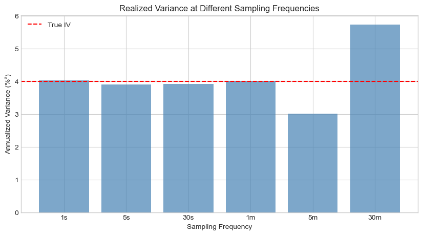

3. Market Microstructure Noise¶

3.1 The Problem¶

Observed prices contain noise from bid-ask bounce, discrete prices, etc.:

p_t^{obs} = p_t^{*} + \eta_t

(4)

where $\eta_t$ is microstructure noise (often i.i.d. with $E[\eta] = 0$ , $\text{Var}(\eta) = \omega^2$ ).

3.2 Impact on RV¶

With noise, as $M \to \infty$ :

RV_t \to IV_t + 2M\omega^2

(5)

RV explodes at high frequencies due to noise!

def add_microstructure_noise(log_prices, noise_std):
    """Add i.i.d. microstructure noise."""
    noise = np.random.normal(0, noise_std, len(log_prices))
    return log_prices + noise

# Add noise
noise_std = 0.0001  # Typical for liquid stocks
noisy_prices = add_microstructure_noise(log_prices, noise_std)

# Compare RV with and without noise
freqs_extended = [1, 2, 5, 10, 30, 60, 120, 300, 600, 1800]
rv_clean = [compute_rv(log_prices, f) for f in freqs_extended]
rv_noisy = [compute_rv(noisy_prices, f) for f in freqs_extended]

fig, ax = plt.subplots(figsize=(12, 6))
ax.plot(freqs_extended, [rv * 252 * 100 for rv in rv_clean], 'b-o', label='No Noise', linewidth=2)
ax.plot(freqs_extended, [rv * 252 * 100 for rv in rv_noisy], 'r-s', label='With Noise', linewidth=2)
ax.axhline(true_iv * 252 * 100, color='green', linestyle='--', label='True IV')
ax.set_xscale('log')
ax.set_xlabel('Sampling Interval (seconds)')
ax.set_ylabel('Annualized RV (%²)')
ax.set_title('Signature Plot: RV vs Sampling Frequency')
ax.legend()
plt.show()

print("\nThe 'signature plot' shows RV exploding at high frequencies due to noise.")
print("Optimal sampling: 5-minute returns (300 seconds) is a common compromise.")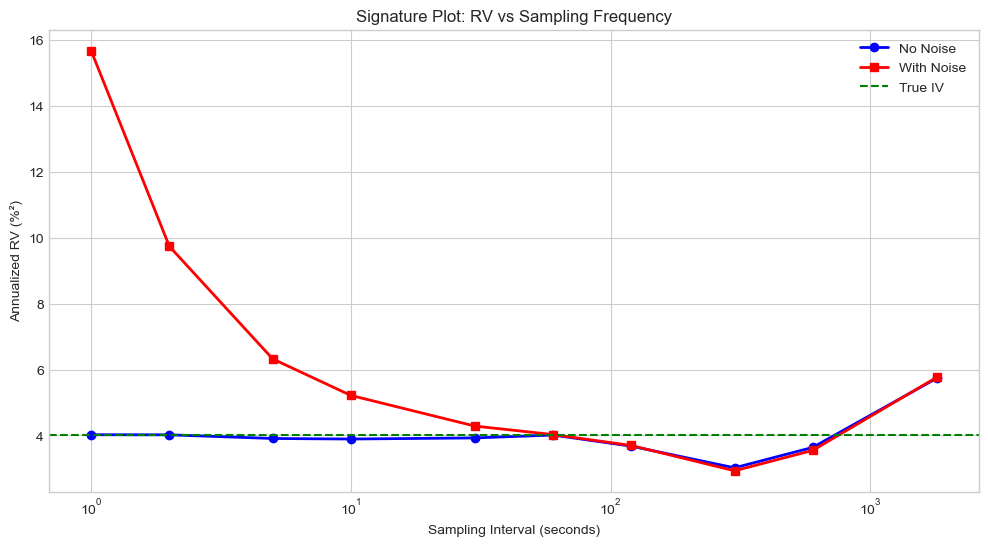


The 'signature plot' shows RV exploding at high frequencies due to noise.
Optimal sampling: 5-minute returns (300 seconds) is a common compromise.

4. Noise-Robust Estimators¶

4.1 Two-Scale Realized Variance (Zhang et al., 2005)¶

TSRV = \frac{1}{K}\sum_{k=1}^{K} RV^{(k)} - \frac{\bar{n}}{n} RV^{(all)}

(6)

4.2 Realized Kernel (Barndorff-Nielsen et al., 2008)¶

RK = \sum_{h=-H}^{H} k\left(\frac{h}{H}\right) \hat{\gamma}_h

(7)

where $\hat{\gamma}_h$ is the autocovariance of returns at lag $h$ .

def two_scale_rv(log_prices, K=5):
    """Two-Scale Realized Variance estimator."""
    n = len(log_prices) - 1
    
    # Slow scale: average of K subsamples
    rv_slow = 0
    for k in range(K):
        subsample = log_prices[k::K]
        returns = np.diff(subsample)
        rv_slow += np.sum(returns**2)
    rv_slow /= K
    
    # Fast scale: all returns
    returns_all = np.diff(log_prices)
    rv_fast = np.sum(returns_all**2)
    
    # Bias correction
    n_bar = (n - K + 1) / K
    tsrv = rv_slow - (n_bar / n) * rv_fast
    
    return max(tsrv, 0)

def realized_kernel(log_prices, H=None, kernel='parzen'):
    """Realized Kernel estimator."""
    returns = np.diff(log_prices)
    n = len(returns)
    
    if H is None:
        H = int(4 * (n/100)**(2/5))
    
    def parzen_kernel(x):
        x = np.abs(x)
        if x <= 0.5:
            return 1 - 6*x**2 + 6*x**3
        elif x <= 1:
            return 2*(1-x)**3
        return 0
    
    # Compute autocovariances
    gamma_0 = np.sum(returns**2)
    rk = gamma_0
    
    for h in range(1, H+1):
        gamma_h = np.sum(returns[h:] * returns[:-h])
        weight = parzen_kernel(h / H)
        rk += 2 * weight * gamma_h
    
    return max(rk, 0)

# Compare estimators
tsrv = two_scale_rv(noisy_prices, K=5)
rk = realized_kernel(noisy_prices)
rv_5min = compute_rv(noisy_prices, 300)

print("Comparison of RV Estimators (with microstructure noise)")
print("="*60)
print(f"True IV (ann.):           {true_iv * 252 * 100:.4f}%²")
print(f"RV 5-minute (ann.):       {rv_5min * 252 * 100:.4f}%²")
print(f"Two-Scale RV (ann.):      {tsrv * 252 * 100:.4f}%²")
print(f"Realized Kernel (ann.):   {rk * 252 * 100:.4f}%²")

Comparison of RV Estimators (with microstructure noise)
============================================================
True IV (ann.):           4.0000%²
RV 5-minute (ann.):       2.9295%²
Two-Scale RV (ann.):      3.0385%²
Realized Kernel (ann.):   3.7773%²

5. Jump-Robust Measures¶

5.1 Bipower Variation¶

BV_t = \mu_1^{-2} \sum_{i=2}^{M} |r_{t,i}| |r_{t,i-1}|

(8)

where $\mu_1 = \sqrt{2/\pi} \approx 0.7979$ . Under no jumps: $BV_t \xrightarrow{p} IV_t$ .

5.2 Jump Detection¶

RV_t - BV_t \xrightarrow{p} \sum_j \kappa_j^2

(9)

where $\kappa_j$ are jump sizes.

def bipower_variation(log_prices, sampling_freq=1):
    """Compute bipower variation."""
    sampled = log_prices[::sampling_freq]
    returns = np.diff(sampled)
    mu1 = np.sqrt(2/np.pi)
    bv = (1/mu1**2) * np.sum(np.abs(returns[1:]) * np.abs(returns[:-1]))
    return bv

def simulate_jump_diffusion(T, n_steps, sigma=0.2, jump_intensity=1, jump_std=0.02, seed=None):
    """Simulate jump-diffusion process."""
    if seed is not None:
        np.random.seed(seed)
    
    dt = T / n_steps
    log_prices = np.zeros(n_steps + 1)
    
    for i in range(n_steps):
        dW = np.random.normal(0, np.sqrt(dt))
        dN = np.random.poisson(jump_intensity * dt)
        jump = np.sum(np.random.normal(0, jump_std, dN)) if dN > 0 else 0
        log_prices[i+1] = log_prices[i] + sigma * dW + jump
    
    return log_prices

# Simulate with jumps
log_prices_jump = simulate_jump_diffusion(T, n_steps, sigma=sigma_true, 
                                          jump_intensity=5, jump_std=0.005, seed=42)

rv_jump = compute_rv(log_prices_jump, 300)
bv_jump = bipower_variation(log_prices_jump, 300)
jump_component = max(rv_jump - bv_jump, 0)

print("Jump Detection using Bipower Variation")
print("="*50)
print(f"RV (5-min):          {rv_jump * 252 * 100:.4f}%² (ann.)")
print(f"BV (5-min):          {bv_jump * 252 * 100:.4f}%² (ann.)")
print(f"Jump Component:      {jump_component * 252 * 100:.4f}%² (ann.)")
print(f"Jump Share:          {100 * jump_component / rv_jump:.1f}%")

Jump Detection using Bipower Variation
==================================================
RV (5-min):          4.1741%² (ann.)
BV (5-min):          3.8990%² (ann.)
Jump Component:      0.2751%² (ann.)
Jump Share:          6.6%

6. Realized Measures: Summary¶

Measure	Formula	Properties
RV	$\sum r_i^2$	Simple, sensitive to noise and jumps
BV	$\mu_1^{-2} \sum	r_i
TSRV	Subsampling + bias correction	Noise-robust
RK	Kernel-weighted autocovariances	Noise-robust

7. Summary¶

Key Takeaways¶

Realized Variance provides a direct measure of volatility from high-frequency data
Microstructure noise causes RV to explode at ultra-high frequencies
Signature plots help identify optimal sampling frequency
Noise-robust estimators (TSRV, RK) enable use of higher frequencies
Bipower variation is robust to jumps

Preview: Session 6¶

HAR models for forecasting realized volatility.

Exercises¶

Implement the median realized variance (MedRV) and compare to BV for jump robustness
Create signature plots for different noise levels
Implement the pre-averaging estimator of Jacod et al. (2009)
Test jump detection using the ratio statistic $RV/BV$

References¶

Andersen, T. G., Bollerslev, T., Diebold, F. X., & Labys, P. (2001). The distribution of realized exchange rate volatility. JASA, 96(453), 42-55.
Barndorff-Nielsen, O. E., & Shephard, N. (2004). Power and bipower variation. Econometrica, 72(5), 1481-1517.
Zhang, L., Mykland, P. A., & Aït-Sahalia, Y. (2005). A tale of two time scales. JASA, 100(472), 1394-1411.