Session 6: Cross-Sectional Analysis
Event Studies in Finance and Economics - Summer School
Learning Objectives
By the end of this session, you will be able to:
Understand why cross-sectional variation in event responses matters
Implement cross-sectional regression analysis of CARs
Handle heteroskedasticity in cross-sectional regressions
Use weighted least squares (WLS) for efficient estimation
Analyze determinants of abnormal returns
Address endogeneity concerns in event study settings
1. Introduction: Beyond Average Effects
From CAAR to Cross-Sectional Analysis
So far, we’ve focused on testing whether the average abnormal return differs from zero. But events often affect firms differently:
Earnings announcements: Surprise magnitude matters
M&A announcements: Deal characteristics affect returns
Regulatory changes: Firm exposure varies
Macroeconomic shocks: Industry and size matter
The Cross-Sectional Regression
Where are firm or event characteristics that may explain variation in abnormal returns.
Key Questions
What firm characteristics predict stronger/weaker event responses?
Do deal characteristics affect announcement returns?
How does prior information affect the market reaction?
Are there systematic patterns across industries or time?
2. Setup and Data
Source
import numpy as np
import pandas as pd
import matplotlib.pyplot as plt
import seaborn as sns
from scipy import stats
import yfinance as yf
import statsmodels.api as sm
from statsmodels.stats.outliers_influence import variance_inflation_factor
from statsmodels.stats.diagnostic import het_breuschpagan, het_white
from datetime import timedelta
from dataclasses import dataclass
from typing import List, Dict, Optional, Tuple
import warnings
warnings.filterwarnings('ignore')

plt.style.use('seaborn-v0_8-whitegrid')
sns.set_palette("husl")
print("Libraries loaded!")
Libraries loaded!
Source
# Extended sample with firm characteristics for cross-sectional analysis
# Using Q2-Q3 2023 earnings announcements with additional firm data
EVENTS = [
    # Tech - Large Cap
    {'ticker': 'AAPL', 'date': '2023-08-03', 'name': 'Apple', 'sector': 'Tech', 'eps_surprise': 0.05},
    {'ticker': 'MSFT', 'date': '2023-07-25', 'name': 'Microsoft', 'sector': 'Tech', 'eps_surprise': 0.08},
    {'ticker': 'GOOGL', 'date': '2023-07-25', 'name': 'Alphabet', 'sector': 'Tech', 'eps_surprise': 0.12},
    {'ticker': 'AMZN', 'date': '2023-08-03', 'name': 'Amazon', 'sector': 'Tech', 'eps_surprise': 0.45},
    {'ticker': 'META', 'date': '2023-07-26', 'name': 'Meta', 'sector': 'Tech', 'eps_surprise': 0.22},
    {'ticker': 'NVDA', 'date': '2023-08-23', 'name': 'Nvidia', 'sector': 'Tech', 'eps_surprise': 0.35},
    # Tech - Smaller
    {'ticker': 'AMD', 'date': '2023-08-01', 'name': 'AMD', 'sector': 'Tech', 'eps_surprise': -0.02},
    {'ticker': 'INTC', 'date': '2023-07-27', 'name': 'Intel', 'sector': 'Tech', 'eps_surprise': 0.18},
    {'ticker': 'CRM', 'date': '2023-08-30', 'name': 'Salesforce', 'sector': 'Tech', 'eps_surprise': 0.15},
    {'ticker': 'ADBE', 'date': '2023-09-14', 'name': 'Adobe', 'sector': 'Tech', 'eps_surprise': 0.06},
    # Finance
    {'ticker': 'JPM', 'date': '2023-07-14', 'name': 'JPMorgan', 'sector': 'Finance', 'eps_surprise': 0.10},
    {'ticker': 'BAC', 'date': '2023-07-18', 'name': 'Bank of America', 'sector': 'Finance', 'eps_surprise': 0.03},
    {'ticker': 'WFC', 'date': '2023-07-14', 'name': 'Wells Fargo', 'sector': 'Finance', 'eps_surprise': 0.08},
    {'ticker': 'GS', 'date': '2023-07-19', 'name': 'Goldman Sachs', 'sector': 'Finance', 'eps_surprise': -0.15},
    {'ticker': 'MS', 'date': '2023-07-18', 'name': 'Morgan Stanley', 'sector': 'Finance', 'eps_surprise': -0.05},
    # Healthcare
    {'ticker': 'JNJ', 'date': '2023-07-20', 'name': 'Johnson & Johnson', 'sector': 'Healthcare', 'eps_surprise': 0.04},
    {'ticker': 'UNH', 'date': '2023-07-14', 'name': 'UnitedHealth', 'sector': 'Healthcare', 'eps_surprise': 0.02},
    {'ticker': 'PFE', 'date': '2023-08-01', 'name': 'Pfizer', 'sector': 'Healthcare', 'eps_surprise': -0.08},
    {'ticker': 'MRK', 'date': '2023-07-27', 'name': 'Merck', 'sector': 'Healthcare', 'eps_surprise': 0.12},
    {'ticker': 'ABBV', 'date': '2023-07-27', 'name': 'AbbVie', 'sector': 'Healthcare', 'eps_surprise': 0.05},
    # Consumer
    {'ticker': 'PG', 'date': '2023-07-28', 'name': 'Procter & Gamble', 'sector': 'Consumer', 'eps_surprise': 0.03},
    {'ticker': 'KO', 'date': '2023-07-26', 'name': 'Coca-Cola', 'sector': 'Consumer', 'eps_surprise': 0.05},
    {'ticker': 'PEP', 'date': '2023-07-13', 'name': 'PepsiCo', 'sector': 'Consumer', 'eps_surprise': 0.07},
    {'ticker': 'WMT', 'date': '2023-08-17', 'name': 'Walmart', 'sector': 'Consumer', 'eps_surprise': 0.09},
    {'ticker': 'COST', 'date': '2023-09-26', 'name': 'Costco', 'sector': 'Consumer', 'eps_surprise': 0.04},
]

EST_WINDOW, GAP, PRE, POST = 120, 10, 5, 5
print(f"Sample: {len(EVENTS)} earnings announcements across {len(set(e['sector'] for e in EVENTS))} sectors")
Sample: 25 earnings announcements across 4 sectors
Source
@dataclass
class EventResult:
    """Container for event study results with firm characteristics."""
    ticker: str
    name: str
    sector: str
    event_date: pd.Timestamp
    eps_surprise: float
    market_cap: float
    beta: float
    sigma: float
    pre_event_return: float
    event_data: pd.DataFrame
    car_var: float  # Variance of CAR for WLS


def get_firm_characteristics(ticker: str) -> Dict:
    """Fetch firm characteristics from Yahoo Finance."""
    try:
        stock = yf.Ticker(ticker)
        info = stock.info
        return {
            'market_cap': info.get('marketCap', np.nan),
            'beta': info.get('beta', np.nan),
        }
    except:
        return {'market_cap': np.nan, 'beta': np.nan}


def process_event(event: Dict, est_window: int, gap: int, pre: int, post: int) -> Optional[EventResult]:
    """Process single event and extract characteristics."""
    try:
        ticker = event['ticker']
        event_dt = pd.to_datetime(event['date'])
        start = event_dt - timedelta(days=int((est_window + gap + pre) * 1.5))
        end = event_dt + timedelta(days=int(post * 2.5))

        stock = yf.download(ticker, start=start, end=end, progress=False)['Close']
        market = yf.download('^GSPC', start=start, end=end, progress=False)['Close']

        df = pd.DataFrame({'stock': stock.squeeze(), 'market': market.squeeze()})
        df['stock_ret'] = df['stock'].pct_change()
        df['market_ret'] = df['market'].pct_change()
        df = df.dropna()

        if event_dt not in df.index:
            idx = df.index.get_indexer([event_dt], method='nearest')[0]
            event_dt = df.index[idx]

        event_idx = df.index.get_loc(event_dt)
        df['event_time'] = range(-event_idx, len(df) - event_idx)

        # Split windows
        est_end = -(gap + pre)
        est_data = df[(df['event_time'] >= est_end - est_window) & (df['event_time'] < est_end)]
        evt_data = df[(df['event_time'] >= -pre) & (df['event_time'] <= post)].copy()

        # Market model estimation
        y, x = est_data['stock_ret'].values, est_data['market_ret'].values
        X = sm.add_constant(x)
        ols = sm.OLS(y, X).fit()

        alpha, beta = ols.params[0], ols.params[1]
        sigma = np.std(ols.resid, ddof=2)

        # Abnormal returns
        evt_data['expected'] = alpha + beta * evt_data['market_ret']
        evt_data['AR'] = evt_data['stock_ret'] - evt_data['expected']

        # Pre-event cumulative return (momentum proxy)
        pre_event_data = df[(df['event_time'] >= -60) & (df['event_time'] < -pre)]
        pre_event_return = (1 + pre_event_data['stock_ret']).prod() - 1 if len(pre_event_data) > 0 else 0

        # CAR variance for WLS
        L = len(evt_data[(evt_data['event_time'] >= -1) & (evt_data['event_time'] <= 1)])
        car_var = L * sigma**2

        # Get firm characteristics
        chars = get_firm_characteristics(ticker)

        return EventResult(
            ticker=ticker,
            name=event['name'],
            sector=event['sector'],
            event_date=event_dt,
            eps_surprise=event['eps_surprise'],
            market_cap=chars['market_cap'],
            beta=beta,
            sigma=sigma,
            pre_event_return=pre_event_return,
            event_data=evt_data,
            car_var=car_var
        )
    except Exception as e:
        print(f"{event['ticker']}: FAILED - {e}")
        return None


print("Processing events...")
event_results = [r for e in EVENTS if (r := process_event(e, EST_WINDOW, GAP, PRE, POST))]
print(f"Successfully processed {len(event_results)} events")
Processing events...
YF.download() has changed argument auto_adjust default to True
Successfully processed 25 events
Source
def calculate_car(event_data: pd.DataFrame, tau1: int, tau2: int) -> float:
    mask = (event_data['event_time'] >= tau1) & (event_data['event_time'] <= tau2)
    return event_data.loc[mask, 'AR'].sum()


# Create cross-sectional dataset
def create_cross_sectional_data(event_results: List[EventResult], tau1: int, tau2: int) -> pd.DataFrame:
    """Create dataset for cross-sectional regression."""
    data = []
    for r in event_results:
        car = calculate_car(r.event_data, tau1, tau2)
        data.append({
            'ticker': r.ticker,
            'name': r.name,
            'sector': r.sector,
            'CAR': car,
            'eps_surprise': r.eps_surprise,
            'log_mcap': np.log(r.market_cap) if r.market_cap and r.market_cap > 0 else np.nan,
            'beta': r.beta,
            'sigma': r.sigma,
            'momentum': r.pre_event_return,
            'car_var': r.car_var,
            'car_se': np.sqrt(r.car_var)
        })

    df = pd.DataFrame(data)
    df = df.dropna()
    return df


# Create dataset for CAR(-1,+1)
cs_data = create_cross_sectional_data(event_results, -1, 1)
print(f"\nCross-sectional dataset: {len(cs_data)} observations")
print(cs_data[['ticker', 'sector', 'CAR', 'eps_surprise', 'log_mcap']].head(10).to_string())
Cross-sectional dataset: 24 observations
  ticker sector       CAR  eps_surprise   log_mcap
0   AAPL   Tech -0.051469          0.05  28.931133
1   MSFT   Tech -0.031932          0.08  28.840995
2  GOOGL   Tech  0.062735          0.12  29.018200
3   AMZN   Tech  0.090422          0.45  28.549368
4   META   Tech  0.060857          0.22  28.121054
5   NVDA   Tech -0.000214          0.35  29.135165
6    AMD   Tech -0.011225         -0.02  26.746914
7   INTC   Tech  0.075252          0.18  26.280505
8    CRM   Tech  0.023052          0.15  26.103816
9   ADBE   Tech -0.026877          0.06  25.555308
3. Exploratory Analysis
Source
# Summary statistics by sector
print("Summary Statistics by Sector:")
print("="*70)

sector_stats = cs_data.groupby('sector').agg({
    'CAR': ['count', 'mean', 'median', 'std'],
    'eps_surprise': 'mean',
    'log_mcap': 'mean'
}).round(4)

sector_stats.columns = ['N', 'Mean CAR', 'Median CAR', 'Std CAR', 'Avg EPS Surp', 'Avg Log MCap']
sector_stats['Mean CAR'] = sector_stats['Mean CAR'].apply(lambda x: f"{x*100:.2f}%")
sector_stats['Median CAR'] = sector_stats['Median CAR'].apply(lambda x: f"{x*100:.2f}%")
sector_stats['Std CAR'] = sector_stats['Std CAR'].apply(lambda x: f"{x*100:.2f}%")
print(sector_stats.to_string())
Summary Statistics by Sector:
======================================================================
N Mean CAR Median CAR Std CAR Avg EPS Surp Avg Log MCap
sector
Consumer 5 0.91% 1.42% 1.03% 0.056 26.6830
Finance 4 4.86% 4.89% 2.81% 0.015 26.7116
Healthcare 5 3.91% 6.73% 4.37% 0.030 26.4434
Tech 10 1.91% 1.14% 5.04% 0.164 27.7282
Source
# Visualize relationships
fig, axes = plt.subplots(2, 2, figsize=(12, 10))

# CAR vs EPS Surprise
ax1 = axes[0, 0]
colors = {'Tech': 'blue', 'Finance': 'green', 'Healthcare': 'red', 'Consumer': 'purple'}
for sector in cs_data['sector'].unique():
    mask = cs_data['sector'] == sector
    ax1.scatter(cs_data.loc[mask, 'eps_surprise'], cs_data.loc[mask, 'CAR']*100,
                label=sector, alpha=0.7, s=80, c=colors.get(sector, 'gray'))

# Add regression line
z = np.polyfit(cs_data['eps_surprise'], cs_data['CAR']*100, 1)
p = np.poly1d(z)
x_line = np.linspace(cs_data['eps_surprise'].min(), cs_data['eps_surprise'].max(), 100)
ax1.plot(x_line, p(x_line), 'k--', alpha=0.7, label='OLS fit')

ax1.set_xlabel('EPS Surprise', fontsize=11)
ax1.set_ylabel('CAR (-1,+1) %', fontsize=11)
ax1.set_title('CAR vs Earnings Surprise', fontsize=12)
ax1.axhline(0, color='gray', linestyle='-', linewidth=0.5)
ax1.axvline(0, color='gray', linestyle='-', linewidth=0.5)
ax1.legend(fontsize=9)

# CAR vs Market Cap
ax2 = axes[0, 1]
ax2.scatter(cs_data['log_mcap'], cs_data['CAR']*100, alpha=0.7, s=80)
z = np.polyfit(cs_data['log_mcap'], cs_data['CAR']*100, 1)
p = np.poly1d(z)
x_line = np.linspace(cs_data['log_mcap'].min(), cs_data['log_mcap'].max(), 100)
ax2.plot(x_line, p(x_line), 'r--', alpha=0.7)
ax2.set_xlabel('Log Market Cap', fontsize=11)
ax2.set_ylabel('CAR (-1,+1) %', fontsize=11)
ax2.set_title('CAR vs Firm Size', fontsize=12)
ax2.axhline(0, color='gray', linestyle='-', linewidth=0.5)

# CAR distribution by sector
ax3 = axes[1, 0]
sector_order = cs_data.groupby('sector')['CAR'].mean().sort_values().index
cs_data['sector_cat'] = pd.Categorical(cs_data['sector'], categories=sector_order, ordered=True)
bp = ax3.boxplot([cs_data[cs_data['sector'] == s]['CAR']*100 for s in sector_order],
                  labels=sector_order, patch_artist=True)
for patch, sector in zip(bp['boxes'], sector_order):
    patch.set_facecolor(colors.get(sector, 'gray'))
    patch.set_alpha(0.6)
ax3.axhline(0, color='red', linestyle='--', alpha=0.7)
ax3.set_ylabel('CAR (-1,+1) %', fontsize=11)
ax3.set_title('CAR Distribution by Sector', fontsize=12)

# CAR vs Pre-event Momentum
ax4 = axes[1, 1]
ax4.scatter(cs_data['momentum']*100, cs_data['CAR']*100, alpha=0.7, s=80)
z = np.polyfit(cs_data['momentum']*100, cs_data['CAR']*100, 1)
p = np.poly1d(z)
x_line = np.linspace(cs_data['momentum'].min()*100, cs_data['momentum'].max()*100, 100)
ax4.plot(x_line, p(x_line), 'r--', alpha=0.7)
ax4.set_xlabel('Pre-Event 60-day Return (%)', fontsize=11)
ax4.set_ylabel('CAR (-1,+1) %', fontsize=11)
ax4.set_title('CAR vs Momentum', fontsize=12)
ax4.axhline(0, color='gray', linestyle='-', linewidth=0.5)
ax4.axvline(0, color='gray', linestyle='-', linewidth=0.5)

plt.tight_layout()
plt.show()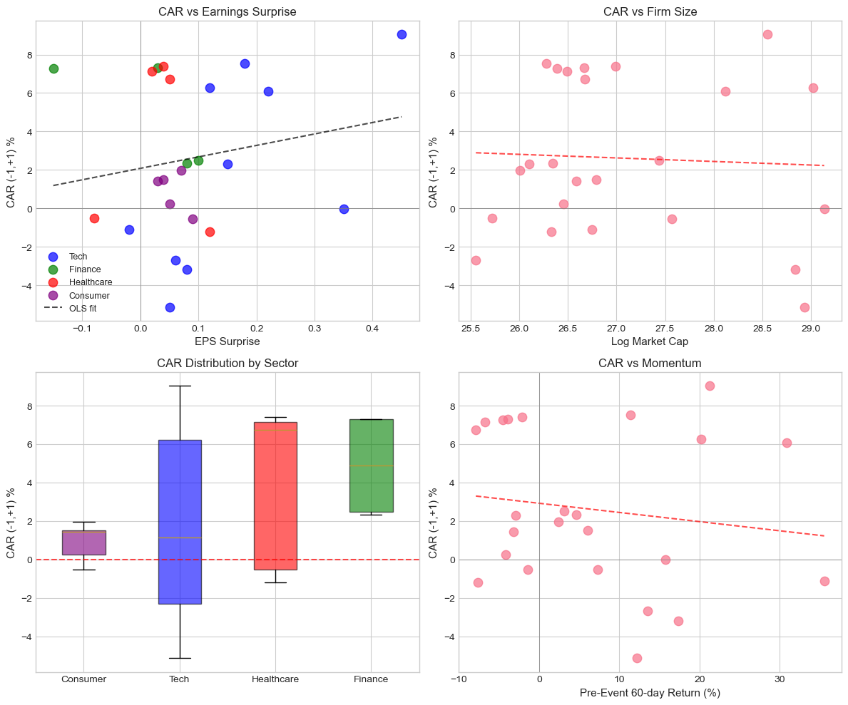
Source
# Correlation matrix
corr_vars = ['CAR', 'eps_surprise', 'log_mcap', 'beta', 'sigma', 'momentum']
corr_matrix = cs_data[corr_vars].corr()

fig, ax = plt.subplots(figsize=(8, 6))
sns.heatmap(corr_matrix, annot=True, fmt='.2f', cmap='RdBu_r', center=0,
            vmin=-1, vmax=1, ax=ax, square=True)
ax.set_title('Correlation Matrix of Cross-Sectional Variables', fontsize=12)
plt.tight_layout()
plt.show()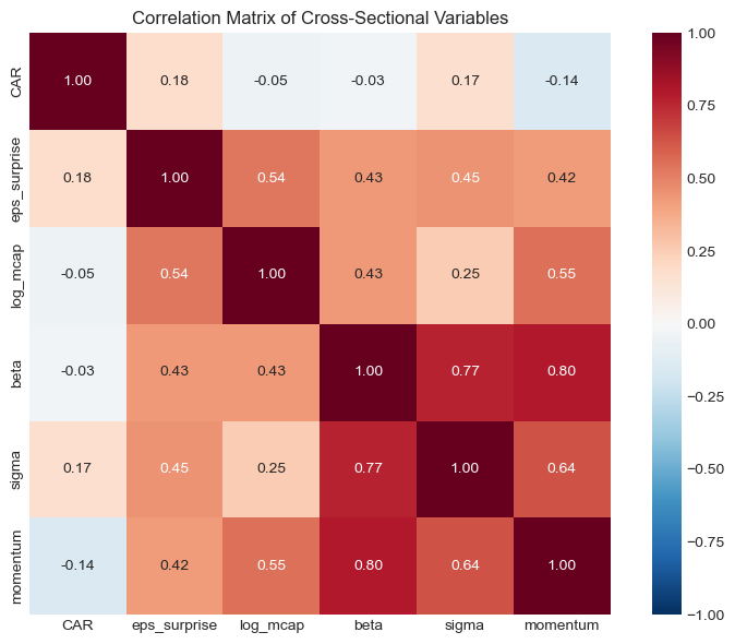
4. Basic OLS Cross-Sectional Regression
Model Specification
Interpretation
: Effect of 1 unit increase in EPS surprise on CAR
: Size effect (do larger firms react differently?)
: Momentum effect (does prior return predict event response?)
Source
def run_cross_sectional_regression(data: pd.DataFrame,
                                    y_var: str,
                                    x_vars: List[str],
                                    add_constant: bool = True) -> sm.regression.linear_model.RegressionResultsWrapper:
    """Run OLS cross-sectional regression."""
    y = data[y_var]
    X = data[x_vars]

    if add_constant:
        X = sm.add_constant(X)

    model = sm.OLS(y, X).fit()
    return model


# Model 1: Simple - EPS Surprise only
print("="*80)
print("MODEL 1: CAR on EPS Surprise")
print("="*80)

model1 = run_cross_sectional_regression(cs_data, 'CAR', ['eps_surprise'])
print(model1.summary())
================================================================================
MODEL 1: CAR on EPS Surprise
================================================================================
OLS Regression Results
==============================================================================
Dep. Variable: CAR R-squared: 0.033
Model: OLS Adj. R-squared: -0.011
Method: Least Squares F-statistic: 0.7415
Date: Fri, 23 Jan 2026 Prob (F-statistic): 0.398
Time: 14:23:42 Log-Likelihood: 43.686
No. Observations: 24 AIC: -83.37
Df Residuals: 22 BIC: -81.02
Df Model: 1
Covariance Type: nonrobust
================================================================================
coef std err t P>|t| [0.025 0.975]
--------------------------------------------------------------------------------
const 0.0208 0.010 2.005 0.057 -0.001 0.042
eps_surprise 0.0596 0.069 0.861 0.398 -0.084 0.203
==============================================================================
Omnibus: 3.483 Durbin-Watson: 1.432
Prob(Omnibus): 0.175 Jarque-Bera (JB): 1.391
Skew: -0.040 Prob(JB): 0.499
Kurtosis: 1.823 Cond. No. 8.35
==============================================================================
Notes:
[1] Standard Errors assume that the covariance matrix of the errors is correctly specified.
Source
# Model 2: Add firm characteristics
print("\n" + "="*80)
print("MODEL 2: CAR on EPS Surprise + Firm Characteristics")
print("="*80)

model2 = run_cross_sectional_regression(cs_data, 'CAR',
                                         ['eps_surprise', 'log_mcap', 'momentum'])
print(model2.summary())
================================================================================
MODEL 2: CAR on EPS Surprise + Firm Characteristics
================================================================================
                            OLS Regression Results
==============================================================================
Dep. Variable:                    CAR   R-squared:                       0.098
Model:                            OLS   Adj. R-squared:                 -0.038
Method:                 Least Squares   F-statistic:                    0.7205
Date:                Fri, 23 Jan 2026   Prob (F-statistic):              0.551
Time:                        14:23:43   Log-Likelihood:                 44.520
No. Observations:                  24   AIC:                            -81.04
Df Residuals:                      20   BIC:                            -76.33
Df Model:                           3
Covariance Type:            nonrobust
================================================================================
                   coef    std err          t      P>|t|      [0.025      0.975]
--------------------------------------------------------------------------------
const            0.1237      0.272      0.455      0.654      -0.443       0.691
eps_surprise     0.1095      0.084      1.297      0.210      -0.067       0.286
log_mcap        -0.0038      0.010     -0.370      0.716      -0.025       0.018
momentum        -0.0757      0.086     -0.876      0.391      -0.256       0.105
==============================================================================
Omnibus:                        6.824   Durbin-Watson:                   1.516
Prob(Omnibus):                  0.033   Jarque-Bera (JB):                1.886
Skew:                           0.089   Prob(JB):                        0.389
Kurtosis:                       1.638   Cond. No.                         885.
==============================================================================

Notes:
[1] Standard Errors assume that the covariance matrix of the errors is correctly specified.
Source
# Model 3: Add sector fixed effects
print("\n" + "="*80)
print("MODEL 3: With Sector Fixed Effects")
print("="*80)

# Create sector dummies
cs_data_fe = cs_data.copy()
sector_dummies = pd.get_dummies(cs_data_fe['sector'], prefix='sector', drop_first=True)
cs_data_fe = pd.concat([cs_data_fe, sector_dummies], axis=1)

x_vars_fe = ['eps_surprise', 'log_mcap', 'momentum'] + list(sector_dummies.columns)
model3 = run_cross_sectional_regression(cs_data_fe, 'CAR', x_vars_fe)
print(model3.summary())
================================================================================
MODEL 3: With Sector Fixed Effects
================================================================================
---------------------------------------------------------------------------
ValueError                                Traceback (most recent call last)
Cell In[26], line 12
      9 cs_data_fe = pd.concat([cs_data_fe, sector_dummies], axis=1)
     11 x_vars_fe = ['eps_surprise', 'log_mcap', 'momentum'] + list(sector_dummies.columns)
---> 12 model3 = run_cross_sectional_regression(cs_data_fe, 'CAR', np.asarray(x_vars_fe))
     13 print(model3.summary())

Cell In[20], line 12, in run_cross_sectional_regression(data, y_var, x_vars, add_constant)
      9 if add_constant:
     10     X = sm.add_constant(X)
---> 12 model = sm.OLS(y, X).fit()
     13 return model

File ~\AppData\Local\anaconda3\Lib\site-packages\statsmodels\regression\linear_model.py:924, in OLS.__init__(self, endog, exog, missing, hasconst, **kwargs)
    921     msg = ("Weights are not supported in OLS and will be ignored"
    922            "An exception will be raised in the next version.")
    923     warnings.warn(msg, ValueWarning)
--> 924 super().__init__(endog, exog, missing=missing,
    925                           hasconst=hasconst, **kwargs)
    926 if "weights" in self._init_keys:
    927     self._init_keys.remove("weights")

File ~\AppData\Local\anaconda3\Lib\site-packages\statsmodels\regression\linear_model.py:749, in WLS.__init__(self, endog, exog, weights, missing, hasconst, **kwargs)
    747 else:
    748     weights = weights.squeeze()
--> 749 super().__init__(endog, exog, missing=missing,
    750                           weights=weights, hasconst=hasconst, **kwargs)
    751 nobs = self.exog.shape[0]
    752 weights = self.weights

File ~\AppData\Local\anaconda3\Lib\site-packages\statsmodels\regression\linear_model.py:203, in RegressionModel.__init__(self, endog, exog, **kwargs)
    202 def __init__(self, endog, exog, **kwargs):
--> 203     super().__init__(endog, exog, **kwargs)
    204     self.pinv_wexog: Float64Array | None = None
    205     self._data_attr.extend(['pinv_wexog', 'wendog', 'wexog', 'weights'])

File ~\AppData\Local\anaconda3\Lib\site-packages\statsmodels\base\model.py:270, in LikelihoodModel.__init__(self, endog, exog, **kwargs)
    269 def __init__(self, endog, exog=None, **kwargs):
--> 270     super().__init__(endog, exog, **kwargs)
    271     self.initialize()

File ~\AppData\Local\anaconda3\Lib\site-packages\statsmodels\base\model.py:95, in Model.__init__(self, endog, exog, **kwargs)
     93 missing = kwargs.pop('missing', 'none')
     94 hasconst = kwargs.pop('hasconst', None)
---> 95 self.data = self._handle_data(endog, exog, missing, hasconst,
     96                               **kwargs)
     97 self.k_constant = self.data.k_constant
     98 self.exog = self.data.exog

File ~\AppData\Local\anaconda3\Lib\site-packages\statsmodels\base\model.py:135, in Model._handle_data(self, endog, exog, missing, hasconst, **kwargs)
    134 def _handle_data(self, endog, exog, missing, hasconst, **kwargs):
--> 135     data = handle_data(endog, exog, missing, hasconst, **kwargs)
    136     # kwargs arrays could have changed, easier to just attach here
    137     for key in kwargs:

File ~\AppData\Local\anaconda3\Lib\site-packages\statsmodels\base\data.py:675, in handle_data(endog, exog, missing, hasconst, **kwargs)
    672     exog = np.asarray(exog)
    674 klass = handle_data_class_factory(endog, exog)
--> 675 return klass(endog, exog=exog, missing=missing, hasconst=hasconst,
    676              **kwargs)

File ~\AppData\Local\anaconda3\Lib\site-packages\statsmodels\base\data.py:84, in ModelData.__init__(self, endog, exog, missing, hasconst, **kwargs)
     82     self.orig_endog = endog
     83     self.orig_exog = exog
---> 84     self.endog, self.exog = self._convert_endog_exog(endog, exog)
     86 self.const_idx = None
     87 self.k_constant = 0

File ~\AppData\Local\anaconda3\Lib\site-packages\statsmodels\base\data.py:509, in PandasData._convert_endog_exog(self, endog, exog)
    507 exog = exog if exog is None else np.asarray(exog)
    508 if endog.dtype == object or exog is not None and exog.dtype == object:
--> 509     raise ValueError("Pandas data cast to numpy dtype of object. "
    510                      "Check input data with np.asarray(data).")
    511 return super()._convert_endog_exog(endog, exog)

ValueError: Pandas data cast to numpy dtype of object. Check input data with np.asarray(data).
Source
['eps_surprise', 'log_mcap', 'momentum'] + list(sector_dummies.columns)['eps_surprise',
'log_mcap',
'momentum',
'sector_Finance',
'sector_Healthcare',
'sector_Tech']5. Heteroskedasticity and Robust Standard Errors
The Problem
In event studies, varies across firms:
Firms with higher idiosyncratic volatility () have noisier CARs
This violates the OLS assumption of homoskedasticity
Testing for Heteroskedasticity
Breusch-Pagan test: Tests if variance depends on regressors
White test: More general test for heteroskedasticity
Solutions
Robust standard errors (White, 1980): Correct SEs without changing coefficients
Weighted Least Squares (WLS): Weight by inverse variance for efficiency
Source
# Test for heteroskedasticity
print("Heteroskedasticity Tests:")
print("="*60)

# Get residuals from Model 2
y = cs_data['CAR']
X = sm.add_constant(cs_data[['eps_surprise', 'log_mcap', 'momentum']])

# Breusch-Pagan test
bp_lm, bp_pval, bp_f, bp_fpval = het_breuschpagan(model2.resid, X)
print(f"\nBreusch-Pagan Test:")
print(f"  LM statistic: {bp_lm:.4f}")
print(f"  p-value: {bp_pval:.4f}")
print(f"  Conclusion: {'Reject H0 - Heteroskedasticity present' if bp_pval < 0.05 else 'Fail to reject H0'}")

# White test
white_lm, white_pval, white_f, white_fpval = het_white(model2.resid, X)
print(f"\nWhite Test:")
print(f"  LM statistic: {white_lm:.4f}")
print(f"  p-value: {white_pval:.4f}")
print(f"  Conclusion: {'Reject H0 - Heteroskedasticity present' if white_pval < 0.05 else 'Fail to reject H0'}")
Heteroskedasticity Tests:
============================================================
Breusch-Pagan Test:
LM statistic: 3.9217
p-value: 0.2700
Conclusion: Fail to reject H0
White Test:
LM statistic: 16.9926
p-value: 0.0488
Conclusion: Reject H0 - Heteroskedasticity present
Source
# Visualize heteroskedasticity
fig, axes = plt.subplots(1, 2, figsize=(12, 5))

# Residuals vs Fitted
ax1 = axes[0]
ax1.scatter(model2.fittedvalues*100, model2.resid*100, alpha=0.7)
ax1.axhline(0, color='red', linestyle='--')
ax1.set_xlabel('Fitted Values (%)', fontsize=11)
ax1.set_ylabel('Residuals (%)', fontsize=11)
ax1.set_title('Residuals vs Fitted Values', fontsize=12)

# Residuals vs Sigma (proxy for heteroskedasticity)
ax2 = axes[1]
ax2.scatter(cs_data['sigma']*100, np.abs(model2.resid)*100, alpha=0.7)
z = np.polyfit(cs_data['sigma']*100, np.abs(model2.resid)*100, 1)
p = np.poly1d(z)
x_line = np.linspace(cs_data['sigma'].min()*100, cs_data['sigma'].max()*100, 100)
ax2.plot(x_line, p(x_line), 'r--', alpha=0.7)
ax2.set_xlabel('Firm Volatility (σ) %', fontsize=11)
ax2.set_ylabel('|Residuals| (%)', fontsize=11)
ax2.set_title('Absolute Residuals vs Volatility', fontsize=12)

plt.tight_layout()
plt.show()

print("\nNote: If residuals spread out with volatility, we have heteroskedasticity.")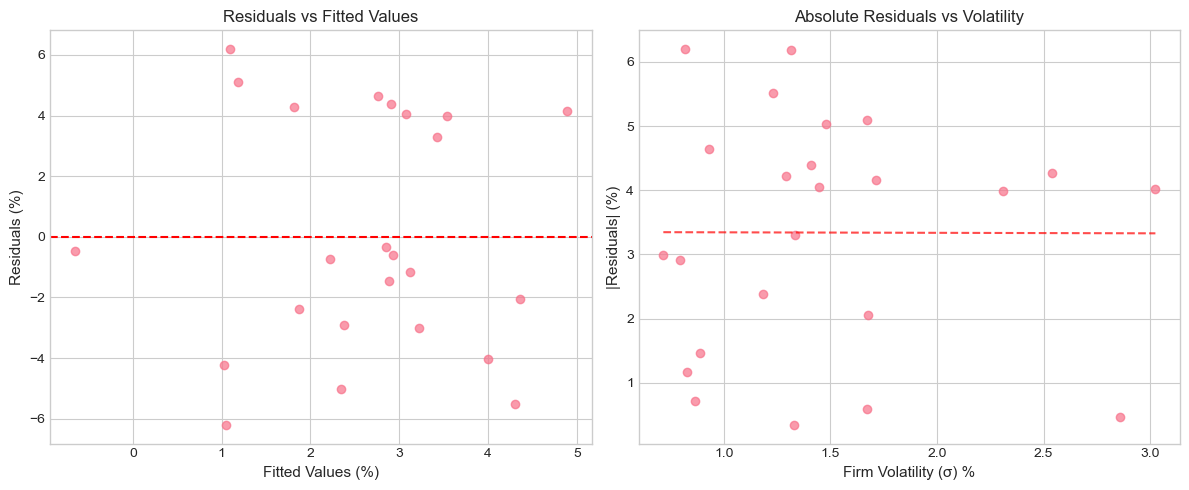
Note: If residuals spread out with volatility, we have heteroskedasticity.
Source
# Compare OLS with Robust Standard Errors
print("\n" + "="*80)
print("COMPARISON: OLS vs Robust Standard Errors")
print("="*80)

# OLS with robust SEs (HC1 = White's heteroskedasticity-consistent)
model2_robust = run_cross_sectional_regression(cs_data, 'CAR',
                                                ['eps_surprise', 'log_mcap', 'momentum'])
model2_robust_hc = model2_robust.get_robustcov_results(cov_type='HC1')

# Create comparison table
comparison = pd.DataFrame({
    'Variable': model2.params.index,
    'Coef': model2.params.values,
    'OLS SE': model2.bse.values,
    'OLS t-stat': model2.tvalues.values,
    'Robust SE': model2_robust_hc.bse,
    'Robust t-stat': model2_robust_hc.tvalues,
})

comparison['SE Change'] = (comparison['Robust SE'] / comparison['OLS SE'] - 1) * 100

print("\nCoefficient Comparison:")
for col in ['Coef', 'OLS SE', 'Robust SE']:
    comparison[col] = comparison[col].apply(lambda x: f"{x:.6f}")
for col in ['OLS t-stat', 'Robust t-stat']:
    comparison[col] = comparison[col].apply(lambda x: f"{x:.3f}")
comparison['SE Change'] = comparison['SE Change'].apply(lambda x: f"{x:+.1f}%")

print(comparison.to_string(index=False))
print("\nNote: Positive SE Change means robust SEs are larger (more conservative).")
================================================================================
COMPARISON: OLS vs Robust Standard Errors
================================================================================

Coefficient Comparison:
    Variable      Coef   OLS SE OLS t-stat Robust SE Robust t-stat SE Change
       const  0.123684 0.271768      0.455  0.324222         0.381    +19.3%
eps_surprise  0.109478 0.084438      1.297  0.098625         1.110    +16.8%
    log_mcap -0.003781 0.010230     -0.370  0.012309        -0.307    +20.3%
    momentum -0.075711 0.086403     -0.876  0.072240        -1.048    -16.4%

Note: Positive SE Change means robust SEs are larger (more conservative).
6. Weighted Least Squares (WLS)
Motivation
When we know the variance structure, WLS is more efficient than OLS with robust SEs.
Weights in Event Studies
Natural weight: inverse of CAR variance
Where is the event window length and is firm i’s residual volatility.
WLS Estimator
Where
Source
def run_wls_regression(data: pd.DataFrame,
                       y_var: str,
                       x_vars: List[str],
                       weight_var: str) -> sm.regression.linear_model.RegressionResultsWrapper:
    """Run Weighted Least Squares regression."""
    y = data[y_var]
    X = sm.add_constant(data[x_vars])

    # Weights = 1/variance (inverse variance weighting)
    weights = 1 / data[weight_var]

    model = sm.WLS(y, X, weights=weights).fit()
    return model


# Run WLS
print("="*80)
print("WEIGHTED LEAST SQUARES (Inverse Variance Weighting)")
print("="*80)

model_wls = run_wls_regression(cs_data, 'CAR',
                                ['eps_surprise', 'log_mcap', 'momentum'],
                                'car_var')
print(model_wls.summary())
================================================================================
WEIGHTED LEAST SQUARES (Inverse Variance Weighting)
================================================================================
WLS Regression Results
==============================================================================
Dep. Variable: CAR R-squared: 0.160
Model: WLS Adj. R-squared: 0.034
Method: Least Squares F-statistic: 1.272
Date: Fri, 23 Jan 2026 Prob (F-statistic): 0.311
Time: 14:25:56 Log-Likelihood: 43.066
No. Observations: 24 AIC: -78.13
Df Residuals: 20 BIC: -73.42
Df Model: 3
Covariance Type: nonrobust
================================================================================
coef std err t P>|t| [0.025 0.975]
--------------------------------------------------------------------------------
const 0.2094 0.281 0.745 0.465 -0.377 0.796
eps_surprise 0.1243 0.105 1.184 0.250 -0.095 0.343
log_mcap -0.0073 0.011 -0.692 0.497 -0.029 0.015
momentum -0.1302 0.124 -1.047 0.307 -0.390 0.129
==============================================================================
Omnibus: 1.108 Durbin-Watson: 1.225
Prob(Omnibus): 0.575 Jarque-Bera (JB): 0.821
Skew: 0.025 Prob(JB): 0.663
Kurtosis: 2.095 Cond. No. 1.01e+03
==============================================================================
Notes:
[1] Standard Errors assume that the covariance matrix of the errors is correctly specified.
[2] The condition number is large, 1.01e+03. This might indicate that there are
strong multicollinearity or other numerical problems.
Source
# Compare OLS, Robust OLS, and WLS
print("\n" + "="*80)
print("COMPARISON: OLS vs Robust OLS vs WLS")
print("="*80)

# Create comprehensive comparison
vars_to_compare = ['const', 'eps_surprise', 'log_mcap', 'momentum']

comparison_full = pd.DataFrame({
    'Variable': vars_to_compare,
    'OLS Coef': [model2.params[v] for v in vars_to_compare],
    'OLS t': [model2.tvalues[v] for v in vars_to_compare],
    'Robust t': [model2_robust_hc.tvalues[v] for v in range(len(vars_to_compare))],
    'WLS Coef': [model_wls.params[v] for v in vars_to_compare],
    'WLS t': [model_wls.tvalues[v] for v in vars_to_compare],
})

def sig(t, df=20):
    p = 2 * (1 - stats.t.cdf(abs(t), df))
    if p < 0.01: return '***'
    elif p < 0.05: return '**'
    elif p < 0.10: return '*'
    return ''

print("\n" + "-"*80)
print(f"{'Variable':<15} {'OLS Coef':>12} {'OLS t':>10} {'Robust t':>10} {'WLS Coef':>12} {'WLS t':>10}")
print("-"*80)
for _, row in comparison_full.iterrows():
    print(f"{row['Variable']:<15} {row['OLS Coef']:>12.6f} {row['OLS t']:>8.2f}{sig(row['OLS t']):2s} "
          f"{row['Robust t']:>8.2f}{sig(row['Robust t']):2s} {row['WLS Coef']:>12.6f} {row['WLS t']:>8.2f}{sig(row['WLS t']):2s}")
print("-"*80)
print(f"{'R-squared':<15} {model2.rsquared:>12.4f} {'':<22} {model_wls.rsquared:>12.4f}")
print(f"{'N':<15} {int(model2.nobs):>12} {'':<22} {int(model_wls.nobs):>12}")
print("\nSignificance: *** p<0.01, ** p<0.05, * p<0.10")
================================================================================
COMPARISON: OLS vs Robust OLS vs WLS
================================================================================

--------------------------------------------------------------------------------
Variable            OLS Coef      OLS t   Robust t     WLS Coef      WLS t
--------------------------------------------------------------------------------
const               0.123684     0.46       0.38       0.209434     0.75
eps_surprise        0.109478     1.30       1.11       0.124321     1.18
log_mcap           -0.003781    -0.37      -0.31      -0.007280    -0.69
momentum           -0.075711    -0.88      -1.05      -0.130245    -1.05
--------------------------------------------------------------------------------
R-squared             0.0975                              0.1602
N                         24                                  24

Significance: *** p<0.01, ** p<0.05, * p<0.10
7. Multicollinearity Diagnostics
Why It Matters
If explanatory variables are highly correlated:
Coefficient estimates become unstable
Standard errors inflate
Hard to isolate individual effects
Variance Inflation Factor (VIF)
Where is from regressing on all other X variables.
Rule of thumb: VIF > 10 suggests serious multicollinearity
Source
def calculate_vif(data: pd.DataFrame, variables: List[str]) -> pd.DataFrame:
    """Calculate Variance Inflation Factors."""
    X = data[variables]
    X = sm.add_constant(X)

    vif_data = []
    for i, var in enumerate(X.columns):
        if var == 'const':
            continue
        vif = variance_inflation_factor(X.values, i)
        vif_data.append({'Variable': var, 'VIF': vif})

    return pd.DataFrame(vif_data)


# Calculate VIFs
print("Multicollinearity Diagnostics:")
print("="*50)

vif_df = calculate_vif(cs_data, ['eps_surprise', 'log_mcap', 'momentum', 'beta', 'sigma'])
vif_df['VIF'] = vif_df['VIF'].apply(lambda x: f"{x:.2f}")
vif_df['Concern'] = vif_df['VIF'].apply(lambda x: 'High' if float(x) > 10 else 'Moderate' if float(x) > 5 else 'Low')

print("\nVariance Inflation Factors:")
print(vif_df.to_string(index=False))
print("\nRule of thumb: VIF > 10 indicates serious multicollinearity")
Multicollinearity Diagnostics:
==================================================
Variance Inflation Factors:
Variable VIF Concern
eps_surprise 1.66 Low
log_mcap 1.88 Low
momentum 3.27 Low
beta 4.11 Low
sigma 2.82 Low
Rule of thumb: VIF > 10 indicates serious multicollinearity
8. Interaction Effects
Research Question
Does the earnings surprise effect vary by firm size? Perhaps smaller firms react more strongly to surprises.
Model with Interaction
: Larger firms react less to surprises
: Larger firms react more to surprises
Source
# Create interaction term
cs_data['surprise_x_size'] = cs_data['eps_surprise'] * cs_data['log_mcap']

# Model with interaction
print("="*80)
print("MODEL WITH INTERACTION: Does Surprise Effect Vary by Size?")
print("="*80)

model_interact = run_cross_sectional_regression(
    cs_data, 'CAR',
    ['eps_surprise', 'log_mcap', 'surprise_x_size', 'momentum']
)
print(model_interact.summary())
================================================================================
MODEL WITH INTERACTION: Does Surprise Effect Vary by Size?
================================================================================
OLS Regression Results
==============================================================================
Dep. Variable: CAR R-squared: 0.120
Model: OLS Adj. R-squared: -0.065
Method: Least Squares F-statistic: 0.6485
Date: Fri, 23 Jan 2026 Prob (F-statistic): 0.635
Time: 14:27:01 Log-Likelihood: 44.824
No. Observations: 24 AIC: -79.65
Df Residuals: 19 BIC: -73.76
Df Model: 4
Covariance Type: nonrobust
===================================================================================
coef std err t P>|t| [0.025 0.975]
-----------------------------------------------------------------------------------
const 0.2542 0.333 0.764 0.454 -0.442 0.951
eps_surprise -1.1918 1.865 -0.639 0.530 -5.096 2.712
log_mcap -0.0086 0.012 -0.691 0.498 -0.035 0.017
surprise_x_size 0.0469 0.067 0.698 0.493 -0.094 0.188
momentum -0.0772 0.088 -0.881 0.389 -0.260 0.106
==============================================================================
Omnibus: 8.908 Durbin-Watson: 1.659
Prob(Omnibus): 0.012 Jarque-Bera (JB): 2.088
Skew: 0.065 Prob(JB): 0.352
Kurtosis: 1.561 Cond. No. 5.96e+03
==============================================================================
Notes:
[1] Standard Errors assume that the covariance matrix of the errors is correctly specified.
[2] The condition number is large, 5.96e+03. This might indicate that there are
strong multicollinearity or other numerical problems.
Source
# Visualize interaction effect
fig, ax = plt.subplots(figsize=(10, 6))

# Split by size (median)
median_mcap = cs_data['log_mcap'].median()
small = cs_data[cs_data['log_mcap'] < median_mcap]
large = cs_data[cs_data['log_mcap'] >= median_mcap]

# Scatter plots
ax.scatter(small['eps_surprise'], small['CAR']*100, color='blue', alpha=0.7,
           s=80, label=f'Small firms (n={len(small)})')
ax.scatter(large['eps_surprise'], large['CAR']*100, color='red', alpha=0.7,
           s=80, label=f'Large firms (n={len(large)})')

# Separate regression lines
for data, color, label in [(small, 'blue', 'Small'), (large, 'red', 'Large')]:
    if len(data) > 2:
        z = np.polyfit(data['eps_surprise'], data['CAR']*100, 1)
        p = np.poly1d(z)
        x_line = np.linspace(data['eps_surprise'].min(), data['eps_surprise'].max(), 100)
        ax.plot(x_line, p(x_line), f'{color[0]}--', linewidth=2, alpha=0.7)

ax.axhline(0, color='gray', linestyle='-', linewidth=0.5)
ax.axvline(0, color='gray', linestyle='-', linewidth=0.5)
ax.set_xlabel('EPS Surprise', fontsize=12)
ax.set_ylabel('CAR (-1,+1) %', fontsize=12)
ax.set_title('Earnings Response: Small vs Large Firms', fontsize=14)
ax.legend()

plt.tight_layout()
plt.show()

# Report slope differences
if len(small) > 2 and len(large) > 2:
    slope_small = np.polyfit(small['eps_surprise'], small['CAR'], 1)[0]
    slope_large = np.polyfit(large['eps_surprise'], large['CAR'], 1)[0]
    print(f"\nEarnings Response Coefficient:")
    print(f"  Small firms: {slope_small:.4f} ({slope_small*100:.2f}% CAR per unit surprise)")
    print(f"  Large firms: {slope_large:.4f} ({slope_large*100:.2f}% CAR per unit surprise)")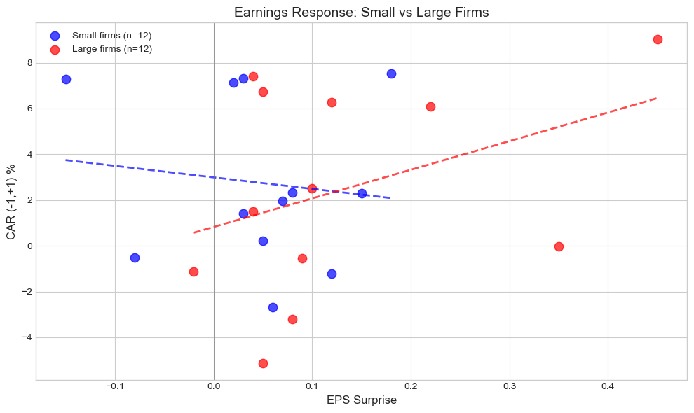
Earnings Response Coefficient:
  Small firms: -0.0503 (-5.03% CAR per unit surprise)
  Large firms: 0.1251 (12.51% CAR per unit surprise)
9. Subsample Analysis
Splitting the Sample
Sometimes relationships differ across subgroups:
Positive vs negative surprises
Different sectors
Different time periods
Source
# Subsample: Positive vs Negative Surprises
print("="*80)
print("SUBSAMPLE ANALYSIS: Positive vs Negative Surprises")
print("="*80)

pos_surprise = cs_data[cs_data['eps_surprise'] > 0]
neg_surprise = cs_data[cs_data['eps_surprise'] <= 0]

print(f"\nPositive surprises: n={len(pos_surprise)}, Mean CAR={pos_surprise['CAR'].mean()*100:.2f}%")
print(f"Negative surprises: n={len(neg_surprise)}, Mean CAR={neg_surprise['CAR'].mean()*100:.2f}%")

# Run regressions on subsamples
if len(pos_surprise) > 5:
    model_pos = run_cross_sectional_regression(pos_surprise, 'CAR', ['eps_surprise', 'log_mcap'])
    print(f"\nPositive Surprise Subsample:")
    print(f"  EPS coefficient: {model_pos.params['eps_surprise']:.4f} (t={model_pos.tvalues['eps_surprise']:.2f})")

if len(neg_surprise) > 5:
    model_neg = run_cross_sectional_regression(neg_surprise, 'CAR', ['eps_surprise', 'log_mcap'])
    print(f"\nNegative Surprise Subsample:")
    print(f"  EPS coefficient: {model_neg.params['eps_surprise']:.4f} (t={model_neg.tvalues['eps_surprise']:.2f})")
================================================================================
SUBSAMPLE ANALYSIS: Positive vs Negative Surprises
================================================================================
Positive surprises: n=21, Mean CAR=2.71%
Negative surprises: n=3, Mean CAR=1.88%
Positive Surprise Subsample:
EPS coefficient: 0.1402 (t=1.48)
Source
# Subsample: By Sector
print("\n" + "="*80)
print("SUBSAMPLE ANALYSIS: By Sector")
print("="*80)

sector_results = []
for sector in cs_data['sector'].unique():
    sector_data = cs_data[cs_data['sector'] == sector]

    if len(sector_data) >= 4:
        try:
            model = run_cross_sectional_regression(sector_data, 'CAR', ['eps_surprise'])
            sector_results.append({
                'Sector': sector,
                'N': len(sector_data),
                'Mean CAR': sector_data['CAR'].mean(),
                'EPS Coef': model.params['eps_surprise'],
                't-stat': model.tvalues['eps_surprise'],
                'R-squared': model.rsquared
            })
        except:
            pass

sector_df = pd.DataFrame(sector_results)
sector_df['Mean CAR'] = sector_df['Mean CAR'].apply(lambda x: f"{x*100:.2f}%")
sector_df['EPS Coef'] = sector_df['EPS Coef'].apply(lambda x: f"{x:.4f}")
sector_df['t-stat'] = sector_df['t-stat'].apply(lambda x: f"{x:.2f}")
sector_df['R-squared'] = sector_df['R-squared'].apply(lambda x: f"{x:.3f}")

print("\nEarnings Response by Sector:")
print(sector_df.to_string(index=False))
================================================================================
SUBSAMPLE ANALYSIS: By Sector
================================================================================

Earnings Response by Sector:
    Sector  N Mean CAR EPS Coef t-stat R-squared
      Tech 10    1.91%   0.2184   2.26     0.389
   Finance  4    4.86%  -0.1867  -1.63     0.572
Healthcare  5    3.91%   0.0405   0.12     0.004
  Consumer  5    0.91%  -0.2298  -1.10     0.286
10. Standardized CAR Regressions
Alternative Approach
Instead of using CAR as dependent variable, use Standardized CAR (SCAR):
This makes the dependent variable unit-free and comparable across firms with different volatilities.
Source
# Create SCAR variable
cs_data['SCAR'] = cs_data['CAR'] / cs_data['car_se']

print("="*80)
print("SCAR REGRESSION (Standardized Dependent Variable)")
print("="*80)

model_scar = run_cross_sectional_regression(cs_data, 'SCAR',
                                             ['eps_surprise', 'log_mcap', 'momentum'])
print(model_scar.summary())
================================================================================
SCAR REGRESSION (Standardized Dependent Variable)
================================================================================
OLS Regression Results
==============================================================================
Dep. Variable: SCAR R-squared: 0.115
Model: OLS Adj. R-squared: -0.017
Method: Least Squares F-statistic: 0.8685
Date: Fri, 23 Jan 2026 Prob (F-statistic): 0.474
Time: 14:27:18 Log-Likelihood: -46.455
No. Observations: 24 AIC: 100.9
Df Residuals: 20 BIC: 105.6
Df Model: 3
Covariance Type: nonrobust
================================================================================
coef std err t P>|t| [0.025 0.975]
--------------------------------------------------------------------------------
const 7.3942 12.035 0.614 0.546 -17.710 32.498
eps_surprise 3.5539 3.739 0.950 0.353 -4.246 11.354
log_mcap -0.2378 0.453 -0.525 0.605 -1.183 0.707
momentum -4.3966 3.826 -1.149 0.264 -12.378 3.585
==============================================================================
Omnibus: 0.047 Durbin-Watson: 1.264
Prob(Omnibus): 0.977 Jarque-Bera (JB): 0.213
Skew: -0.087 Prob(JB): 0.899
Kurtosis: 2.572 Cond. No. 885.
==============================================================================
Notes:
[1] Standard Errors assume that the covariance matrix of the errors is correctly specified.
Source
# Compare CAR vs SCAR regressions
print("\n" + "="*70)
print("COMPARISON: CAR vs SCAR as Dependent Variable")
print("="*70)

print("\nNote: SCAR regression gives t-statistics directly comparable to")
print("standardized test statistics from Sessions 4-5.")
print(f"\nMean SCAR in sample: {cs_data['SCAR'].mean():.3f}")
print(f"Std SCAR: {cs_data['SCAR'].std():.3f}")
print(f"\nIf SCAR ~ N(0,1) under null, mean significantly > 0 indicates positive abnormal returns.")
======================================================================
COMPARISON: CAR vs SCAR as Dependent Variable
======================================================================

Note: SCAR regression gives t-statistics directly comparable to
standardized test statistics from Sessions 4-5.

Mean SCAR in sample: 0.985
Std SCAR: 1.821

If SCAR ~ N(0,1) under null, mean significantly > 0 indicates positive abnormal returns.
11. Addressing Potential Endogeneity
The Problem
In some event studies, explanatory variables may be endogenous:
Reverse causality: Does the event response cause the characteristic?
Omitted variables: Unobserved factors affecting both X and CAR
Measurement error: Noisy proxies for true variables
Example: Earnings Surprise
Management may manage earnings based on expected market reaction
Analysts may adjust forecasts based on anticipated news
Solutions
Use lagged/predetermined variables: Characteristics measured before event
Instrumental Variables: Find exogenous instruments
Natural experiments: Events that are plausibly exogenous
Source
# Demonstrate using pre-determined variables
print("="*80)
print("ADDRESSING ENDOGENEITY: Using Pre-Determined Variables")
print("="*80)

print("\nVariables in our model and their timing:")
print("-" * 60)
print("  eps_surprise:  Realized at event (potentially endogenous)")
print("  log_mcap:      Measured before event (pre-determined)")
print("  momentum:      60-day pre-event return (pre-determined)")
print("  beta:          Estimated from pre-event data (pre-determined)")
print("  sigma:         Estimated from pre-event data (pre-determined)")

# Model using only pre-determined variables
print("\nModel with only pre-determined variables:")
model_predet = run_cross_sectional_regression(cs_data, 'CAR',
                                               ['log_mcap', 'momentum', 'beta', 'sigma'])
print(f"R-squared: {model_predet.rsquared:.4f}")
print(f"\nNote: Low R-squared without eps_surprise suggests surprise")
print("      is the main driver, as expected for earnings announcements.")
================================================================================
ADDRESSING ENDOGENEITY: Using Pre-Determined Variables
================================================================================
Variables in our model and their timing:
------------------------------------------------------------
eps_surprise: Realized at event (potentially endogenous)
log_mcap: Measured before event (pre-determined)
momentum: 60-day pre-event return (pre-determined)
beta: Estimated from pre-event data (pre-determined)
sigma: Estimated from pre-event data (pre-determined)
Model with only pre-determined variables:
R-squared: 0.1461
Note: Low R-squared without eps_surprise suggests surprise
is the main driver, as expected for earnings announcements.
12. Publication-Ready Results
Source
def create_regression_table(models: List, model_names: List[str],
                            var_order: List[str]) -> pd.DataFrame:
    """Create publication-style regression table."""
    rows = []

    for var in var_order:
        coef_row = {'Variable': var}
        se_row = {'Variable': ''}

        for model, name in zip(models, model_names):
            if var in model.params.index:
                coef = model.params[var]
                se = model.bse[var]
                t = model.tvalues[var]
                p = model.pvalues[var]

                sig = '***' if p < 0.01 else '**' if p < 0.05 else '*' if p < 0.10 else ''
                coef_row[name] = f"{coef:.4f}{sig}"
                se_row[name] = f"({se:.4f})"
            else:
                coef_row[name] = ''
                se_row[name] = ''

        rows.append(coef_row)
        rows.append(se_row)

    # Add statistics
    rows.append({'Variable': ''})

    r2_row = {'Variable': 'R-squared'}
    n_row = {'Variable': 'N'}

    for model, name in zip(models, model_names):
        r2_row[name] = f"{model.rsquared:.3f}"
        n_row[name] = f"{int(model.nobs)}"

    rows.append(r2_row)
    rows.append(n_row)

    return pd.DataFrame(rows)


# Create table
print("\n" + "="*90)
print("TABLE: Cross-Sectional Determinants of Earnings Announcement Returns")
print("="*90)
print("Dependent Variable: CAR(-1,+1)")
print("-"*90)

models = [model1, model2, model_wls, model_interact]
names = ['(1)', '(2) OLS', '(3) WLS', '(4) Interact']
var_order = ['const', 'eps_surprise', 'log_mcap', 'momentum', 'surprise_x_size']

table = create_regression_table(models, names, var_order)
print(table.to_string(index=False))
print("-"*90)
print("Standard errors in parentheses. *** p<0.01, ** p<0.05, * p<0.10")
print("WLS uses inverse CAR variance as weights.")
==========================================================================================
TABLE: Cross-Sectional Determinants of Earnings Announcement Returns
==========================================================================================
Dependent Variable: CAR(-1,+1)
------------------------------------------------------------------------------------------
       Variable      (1)  (2) OLS  (3) WLS (4) Interact
          const  0.0208*   0.1237   0.2094       0.2542
                (0.0104) (0.2718) (0.2810)     (0.3328)
   eps_surprise   0.0596   0.1095   0.1243      -1.1918
                (0.0692) (0.0844) (0.1050)     (1.8653)
       log_mcap           -0.0038  -0.0073      -0.0086
                         (0.0102) (0.0105)     (0.0125)
       momentum           -0.0757  -0.1302      -0.0772
                         (0.0864) (0.1244)     (0.0876)
surprise_x_size                                  0.0469
                                               (0.0672)
                     NaN      NaN      NaN          NaN
      R-squared    0.033    0.098    0.160        0.120
              N       24       24       24           24
------------------------------------------------------------------------------------------
Standard errors in parentheses. *** p<0.01, ** p<0.05, * p<0.10
WLS uses inverse CAR variance as weights.
13. Exercises
Exercise 1: Additional Variables
Add analyst coverage (number of analysts) as an explanatory variable. Does it affect the earnings response?
Exercise 2: Non-Linear Effects
Test for non-linear effects by adding squared terms or using splines.
Exercise 3: Clustered Standard Errors
Implement standard errors clustered by sector or event date.
Source
# Exercise 3: Clustered Standard Errors
print("Exercise 3: Clustered Standard Errors")
print("="*60)

# Cluster by sector
y = cs_data['CAR']
X = sm.add_constant(cs_data[['eps_surprise', 'log_mcap', 'momentum']])

# OLS with clustered SEs by sector
model_cluster = sm.OLS(y, X).fit(cov_type='cluster',
                                  cov_kwds={'groups': cs_data['sector']})

print("\nOLS with Standard Errors Clustered by Sector:")
print("-"*60)
print(f"{'Variable':<15} {'Coef':>12} {'Clustered SE':>14} {'t-stat':>10}")
print("-"*60)
for var in model_cluster.params.index:
    coef = model_cluster.params[var]
    se = model_cluster.bse[var]
    t = model_cluster.tvalues[var]
    print(f"{var:<15} {coef:>12.6f} {se:>14.6f} {t:>10.2f}")
Exercise 3: Clustered Standard Errors
============================================================
OLS with Standard Errors Clustered by Sector:
------------------------------------------------------------
Variable Coef Clustered SE t-stat
------------------------------------------------------------
const 0.123684 0.239558 0.52
eps_surprise 0.109478 0.110609 0.99
log_mcap -0.003781 0.009481 -0.40
momentum -0.075711 0.059479 -1.27
14. Summary
Key Takeaways
Cross-sectional analysis reveals why events affect firms differently
Heteroskedasticity is common in event studies; use robust SEs or WLS
WLS with inverse variance weights is efficient when variance structure is known
Check for multicollinearity using VIF before interpreting coefficients
Interaction effects can reveal whether relationships vary across subgroups
Endogeneity may bias results; use pre-determined variables when possible
Best Practices
Report both OLS and robust SEs
Consider WLS when variance estimates are reliable
Test for heteroskedasticity explicitly
Run subsample analyses for robustness
Be cautious about endogeneity in event characteristics
Coming Up Next
Session 7: Long-Horizon Event Studies will cover:
Calendar-time portfolio approach
Buy-and-hold abnormal returns (BHAR)
Dealing with overlapping events
Power issues in long-horizon studies
References
White, H. (1980). A heteroskedasticity-consistent covariance matrix estimator and a direct test for heteroskedasticity. Econometrica, 48(4), 817-838.
MacKinnon, J. G., & White, H. (1985). Some heteroskedasticity-consistent covariance matrix estimators with improved finite sample properties. Journal of Econometrics, 29(3), 305-325.
Kothari, S. P., & Warner, J. B. (2007). Econometrics of event studies. Handbook of Corporate Finance, 1, 3-36.
Prabhala, N. R. (1997). Conditional methods in event studies and an equilibrium justification for standard event-study procedures. Review of Financial Studies, 10(1), 1-38.