Session 4: Statistical Inference I - Parametric Tests
Event Studies in Finance and Economics - Summer School
Learning Objectives
By the end of this session, you will be able to:
Understand the assumptions underlying parametric event study tests
Implement and interpret the standard t-test for event studies
Apply the Patell (1976) standardized residual test
Use the Boehmer, Musumeci, and Poulsen (1991) test for event-induced variance
Distinguish between cross-sectional and time-series variance approaches
Evaluate the power and specification of different test statistics
1. Introduction: The Inference Problem
From Measurement to Inference
In Session 3, we learned how to measure abnormal returns. But measurement alone doesn’t tell us whether the event had a statistically significant effect. We need formal hypothesis tests.
The Null Hypothesis
Key Challenges
Estimation error: Parameters (, ) are estimated, not known
Cross-sectional correlation: Events may cluster in calendar time
Event-induced variance: The event itself may change volatility
Non-normality: Returns are often fat-tailed
Small samples: Limited number of events in many studies
This session focuses on parametric tests that assume (approximately) normal distributions. Session 5 will cover non-parametric alternatives.
2. Setup and Data
Source
import numpy as np
import pandas as pd
import matplotlib.pyplot as plt
import seaborn as sns
from scipy import stats
from scipy.special import comb
import yfinance as yf
import statsmodels.api as sm
from datetime import datetime, timedelta
from typing import List, Dict, Tuple, Optional
from dataclasses import dataclass
import warnings
warnings.filterwarnings('ignore')

plt.style.use('seaborn-v0_8-whitegrid')
sns.set_palette("husl")

print("Libraries loaded successfully!")
Libraries loaded successfully!
Source
# We'll use a larger sample for better demonstration of test properties
EVENTS = [
    # Tech earnings Q2-Q3 2023
    {'ticker': 'AAPL', 'date': '2023-08-03', 'name': 'Apple Q3'},
    {'ticker': 'MSFT', 'date': '2023-07-25', 'name': 'Microsoft Q4'},
    {'ticker': 'GOOGL', 'date': '2023-07-25', 'name': 'Alphabet Q2'},
    {'ticker': 'AMZN', 'date': '2023-08-03', 'name': 'Amazon Q2'},
    {'ticker': 'META', 'date': '2023-07-26', 'name': 'Meta Q2'},
    {'ticker': 'NVDA', 'date': '2023-08-23', 'name': 'Nvidia Q2'},
    {'ticker': 'TSLA', 'date': '2023-07-19', 'name': 'Tesla Q2'},
    {'ticker': 'AMD', 'date': '2023-08-01', 'name': 'AMD Q2'},
    {'ticker': 'INTC', 'date': '2023-07-27', 'name': 'Intel Q2'},
    {'ticker': 'CRM', 'date': '2023-08-30', 'name': 'Salesforce Q2'},
]

ESTIMATION_WINDOW = 120
GAP = 10
EVENT_WINDOW_PRE = 10
EVENT_WINDOW_POST = 10

print(f"Sample: {len(EVENTS)} tech earnings announcements")
Sample: 10 tech earnings announcements
Source
@dataclass
class MarketModelResults:
    """Container for market model estimation results."""
    alpha: float
    beta: float
    sigma: float
    r_squared: float
    n_obs: int
    market_mean: float
    market_var: float
    residuals: np.ndarray


@dataclass
class EventStudyResult:
    """Container for single event study results."""
    ticker: str
    name: str
    event_date: pd.Timestamp
    model: MarketModelResults
    event_data: pd.DataFrame
    estimation_data: pd.DataFrame


def download_and_process_event(ticker: str, event_date: str, name: str,
                                est_window: int, gap: int,
                                pre: int, post: int) -> Optional[EventStudyResult]:
    """
    Download data and estimate market model for a single event.
    """
    try:
        event_dt = pd.to_datetime(event_date)
        start_date = event_dt - timedelta(days=int((est_window + gap + pre) * 1.5))
        end_date = event_dt + timedelta(days=int(post * 2.5))

        stock = yf.download(ticker, start=start_date, end=end_date, progress=False)['Close']
        market = yf.download('^GSPC', start=start_date, end=end_date, progress=False)['Close']

        df = pd.DataFrame({
            'stock_price': stock.squeeze(),
            'market_price': market.squeeze()
        })

        df['stock_ret'] = df['stock_price'].pct_change()
        df['market_ret'] = df['market_price'].pct_change()
        df = df.dropna()

        if event_dt not in df.index:
            idx = df.index.get_indexer([event_dt], method='nearest')[0]
            event_dt = df.index[idx]

        event_idx = df.index.get_loc(event_dt)
        df['event_time'] = range(-event_idx, len(df) - event_idx)

        # Split windows
        est_end = -(gap + pre)
        est_start = est_end - est_window

        est_data = df[(df['event_time'] >= est_start) & (df['event_time'] < est_end)].copy()
        evt_data = df[(df['event_time'] >= -pre) & (df['event_time'] <= post)].copy()

        # Estimate market model
        y = est_data['stock_ret'].values
        x = est_data['market_ret'].values
        X = sm.add_constant(x)
        ols = sm.OLS(y, X).fit()

        model = MarketModelResults(
            alpha=ols.params[0],
            beta=ols.params[1],
            sigma=np.std(ols.resid, ddof=2),
            r_squared=ols.rsquared,
            n_obs=len(y),
            market_mean=np.mean(x),
            market_var=np.sum((x - np.mean(x))**2),
            residuals=ols.resid
        )

        # Calculate abnormal returns
        evt_data['expected_ret'] = model.alpha + model.beta * evt_data['market_ret']
        evt_data['AR'] = evt_data['stock_ret'] - evt_data['expected_ret']

        return EventStudyResult(
            ticker=ticker,
            name=name,
            event_date=event_dt,
            model=model,
            event_data=evt_data,
            estimation_data=est_data
        )

    except Exception as e:
        print(f"  {ticker}: FAILED - {e}")
        return None


# Process all events
print("Processing events...")
event_results = []
for event in EVENTS:
    result = download_and_process_event(
        event['ticker'], event['date'], event['name'],
        ESTIMATION_WINDOW, GAP, EVENT_WINDOW_PRE, EVENT_WINDOW_POST
    )
    if result:
        event_results.append(result)
        print(f"  {result.ticker}: OK (beta={result.model.beta:.3f}, sigma={result.model.sigma:.4f})")

print(f"\nSuccessfully processed {len(event_results)} events")
Processing events...
YF.download() has changed argument auto_adjust default to True
AAPL: OK (beta=1.127, sigma=0.0080)
MSFT: OK (beta=1.249, sigma=0.0140)
GOOGL: OK (beta=1.404, sigma=0.0166)
AMZN: OK (beta=1.521, sigma=0.0175)
META: OK (beta=1.891, sigma=0.0256)
NVDA: OK (beta=2.068, sigma=0.0305)
TSLA: OK (beta=2.163, sigma=0.0334)
AMD: OK (beta=1.770, sigma=0.0290)
INTC: OK (beta=1.304, sigma=0.0230)
CRM: OK (beta=1.078, sigma=0.0173)
Successfully processed 10 events
3. Test 1: Simple Cross-Sectional t-Test
The Simplest Approach
The most basic test treats individual CARs as independent draws and uses their cross-sectional distribution:
Where:
Assumptions
CARs are independent across firms
CARs are identically distributed
CARs are (approximately) normally distributed
Distribution
Under the null:
Source
def calculate_car(event_data: pd.DataFrame, tau1: int, tau2: int) -> float:
    """Calculate Cumulative Abnormal Return for a window."""
    mask = (event_data['event_time'] >= tau1) & (event_data['event_time'] <= tau2)
    return event_data.loc[mask, 'AR'].sum()


def cross_sectional_t_test(event_results: List[EventStudyResult],
                           tau1: int, tau2: int) -> Dict:
    """
    Simple cross-sectional t-test for CAAR.

    H0: E[CAR] = 0

    Returns:
    --------
    Dictionary with test statistics
    """
    # Calculate individual CARs
    cars = np.array([calculate_car(r.event_data, tau1, tau2) for r in event_results])
    N = len(cars)

    # Sample statistics
    caar = np.mean(cars)
    s_car = np.std(cars, ddof=1)
    se = s_car / np.sqrt(N)

    # t-statistic
    t_stat = caar / se if se > 0 else 0

    # p-value (two-tailed)
    p_value = 2 * (1 - stats.t.cdf(abs(t_stat), df=N-1))

    return {
        'test_name': 'Cross-Sectional t-Test',
        'N': N,
        'CAAR': caar,
        'std_dev': s_car,
        'std_error': se,
        't_stat': t_stat,
        'df': N - 1,
        'p_value': p_value,
        'individual_cars': cars
    }


# Run test for standard windows
print("Cross-Sectional t-Test Results:")
print("="*70)

windows = [(-1, +1), (0, 0), (-5, +5), (-10, +10)]

cs_results = []
for tau1, tau2 in windows:
    result = cross_sectional_t_test(event_results, tau1, tau2)
    cs_results.append(result)

    sig = '***' if result['p_value'] < 0.01 else '**' if result['p_value'] < 0.05 else '*' if result['p_value'] < 0.10 else ''

    print(f"\nWindow [{tau1:+d}, {tau2:+d}]:")
    print(f"  CAAR = {result['CAAR']*100:+.3f}%")
    print(f"  Std. Dev. = {result['std_dev']*100:.3f}%")
    print(f"  t-stat = {result['t_stat']:.3f} {sig}")
    print(f"  p-value = {result['p_value']:.4f}")

print("\n" + "="*70)
print("Significance: * p<0.10, ** p<0.05, *** p<0.01")
Cross-Sectional t-Test Results:
======================================================================
Window [-1, +1]:
CAAR = +0.959%
Std. Dev. = 6.380%
t-stat = 0.475
p-value = 0.6459
Window [+0, +0]:
CAAR = +0.600%
Std. Dev. = 1.223%
t-stat = 1.550
p-value = 0.1556
Window [-5, +5]:
CAAR = -0.761%
Std. Dev. = 6.559%
t-stat = -0.367
p-value = 0.7223
Window [-10, +10]:
CAAR = -5.226%
Std. Dev. = 7.930%
t-stat = -2.084 *
p-value = 0.0669
======================================================================
Significance: * p<0.10, ** p<0.05, *** p<0.01
Source
# Visualize individual CARs and distribution
fig, axes = plt.subplots(1, 2, figsize=(14, 5))

# Get CAR(-1,+1) results
result = cs_results[0]  # (-1, +1) window
cars = result['individual_cars']
tickers = [r.ticker for r in event_results]

# Bar chart of individual CARs
ax1 = axes[0]
colors = ['green' if c >= 0 else 'red' for c in cars]
bars = ax1.bar(tickers, cars * 100, color=colors, alpha=0.7, edgecolor='black')
ax1.axhline(0, color='black', linewidth=0.5)
ax1.axhline(result['CAAR'] * 100, color='blue', linestyle='--',
            label=f'CAAR = {result["CAAR"]*100:+.2f}%')
ax1.set_ylabel('CAR (-1, +1) %', fontsize=12)
ax1.set_title('Individual CARs', fontsize=14)
ax1.legend()
ax1.tick_params(axis='x', rotation=45)

# Distribution of CARs
ax2 = axes[1]
ax2.hist(cars * 100, bins=8, density=True, alpha=0.7, edgecolor='black', label='Empirical')

# Overlay normal distribution
x = np.linspace(cars.min()*100 - 2, cars.max()*100 + 2, 100)
y = stats.norm.pdf(x, result['CAAR']*100, result['std_dev']*100)
ax2.plot(x, y, 'r-', linewidth=2, label='Normal fit')

ax2.axvline(0, color='black', linestyle='-', linewidth=0.5)
ax2.axvline(result['CAAR']*100, color='blue', linestyle='--', label='Mean')
ax2.set_xlabel('CAR (%)', fontsize=12)
ax2.set_ylabel('Density', fontsize=12)
ax2.set_title('Distribution of CARs', fontsize=14)
ax2.legend()

plt.tight_layout()
plt.show()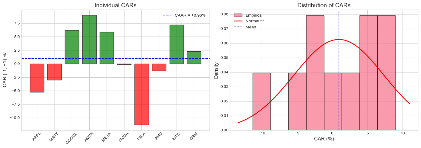
4. Test 2: Time-Series Standard Error Approach
Alternative Variance Estimation
Instead of using cross-sectional variation, we can use the time-series variance from the estimation period:
Where is the length of the event window.
Aggregated Test Statistic
Comparison
| Approach | Variance Source | Pros | Cons |
|---|---|---|---|
| Cross-sectional | Event window | Captures heterogeneity | Needs many events |
| Time-series | Estimation window | Works with few events | Assumes stable variance |
Source
def calculate_car_variance_ts(model: MarketModelResults,
                               event_data: pd.DataFrame,
                               tau1: int, tau2: int) -> float:
    """
    Calculate time-series variance of CAR.

    Includes adjustment for estimation error in alpha and beta.
    """
    mask = (event_data['event_time'] >= tau1) & (event_data['event_time'] <= tau2)
    window_data = event_data[mask]
    L = len(window_data)

    T = model.n_obs
    sigma_sq = model.sigma ** 2
    Rm_bar = model.market_mean
    sum_sq = model.market_var

    # Sum of market return deviations in event window
    Rm_event = window_data['market_ret'].values
    sum_dev_sq = np.sum((Rm_event - Rm_bar) ** 2)

    # Variance formula (Campbell, Lo, MacKinlay 1997, eq. 4.8)
    var = sigma_sq * (L + L**2/T + sum_dev_sq/sum_sq)

    return var


def time_series_t_test(event_results: List[EventStudyResult],
                       tau1: int, tau2: int) -> Dict:
    """
    Time-series variance t-test for CAAR.

    Uses estimation period variance instead of cross-sectional variance.
    """
    cars = []
    car_vars = []

    for r in event_results:
        car = calculate_car(r.event_data, tau1, tau2)
        var = calculate_car_variance_ts(r.model, r.event_data, tau1, tau2)
        cars.append(car)
        car_vars.append(var)

    cars = np.array(cars)
    car_vars = np.array(car_vars)
    N = len(cars)

    caar = np.mean(cars)

    # Time-series aggregated variance
    # Assuming independence: Var(CAAR) = (1/N^2) * sum(Var(CAR_i))
    var_caar = np.sum(car_vars) / (N ** 2)
    se_caar = np.sqrt(var_caar)

    t_stat = caar / se_caar if se_caar > 0 else 0

    # Approximate df (conservative)
    df = N * (ESTIMATION_WINDOW - 2)
    p_value = 2 * (1 - stats.t.cdf(abs(t_stat), df=df))

    return {
        'test_name': 'Time-Series t-Test',
        'N': N,
        'CAAR': caar,
        'var_caar': var_caar,
        'std_error': se_caar,
        't_stat': t_stat,
        'df': df,
        'p_value': p_value,
        'individual_cars': cars,
        'individual_vars': car_vars
    }


# Compare cross-sectional and time-series tests
print("Cross-Sectional vs Time-Series t-Tests:")
print("="*80)

comparison_data = []
for tau1, tau2 in windows:
    cs = cross_sectional_t_test(event_results, tau1, tau2)
    ts = time_series_t_test(event_results, tau1, tau2)

    comparison_data.append({
        'Window': f'[{tau1:+d},{tau2:+d}]',
        'CAAR': cs['CAAR'],
        'CS_SE': cs['std_error'],
        'CS_t': cs['t_stat'],
        'CS_p': cs['p_value'],
        'TS_SE': ts['std_error'],
        'TS_t': ts['t_stat'],
        'TS_p': ts['p_value']
    })

comp_df = pd.DataFrame(comparison_data)

display_comp = comp_df.copy()
display_comp['CAAR'] = display_comp['CAAR'].apply(lambda x: f"{x*100:+.3f}%")
display_comp['CS_SE'] = display_comp['CS_SE'].apply(lambda x: f"{x*100:.3f}%")
display_comp['TS_SE'] = display_comp['TS_SE'].apply(lambda x: f"{x*100:.3f}%")
for col in ['CS_t', 'TS_t']:
    display_comp[col] = display_comp[col].apply(lambda x: f"{x:+.3f}")
for col in ['CS_p', 'TS_p']:
    display_comp[col] = display_comp[col].apply(lambda x: f"{x:.4f}")

print(display_comp.to_string(index=False))
print("\nCS = Cross-Sectional, TS = Time-Series")
Cross-Sectional vs Time-Series t-Tests:
================================================================================
Window CAAR CS_SE CS_t CS_p TS_SE TS_t TS_p
[-1,+1] +0.959% 2.018% +0.475 0.6459 1.271% +0.755 0.4506
[+0,+0] +0.600% 0.387% +1.550 0.1556 0.727% +0.825 0.4095
[-5,+5] -0.761% 2.074% -0.367 0.7223 2.509% -0.303 0.7618
[-10,+10] -5.226% 2.508% -2.084 0.0669 3.595% -1.454 0.1463
CS = Cross-Sectional, TS = Time-Series
5. Test 3: Patell (1976) Standardized Residual Test
Motivation
The simple tests treat all firms equally, but firms have different estimation period variances. Patell’s test standardizes each firm’s abnormal return by its own standard error.
Standardized Abnormal Return
Where:
Standardized CAR
Where:
Patell Test Statistic
Under the null:
Source
def calculate_sar(event_data: pd.DataFrame, model: MarketModelResults) -> np.ndarray:
    """
    Calculate Standardized Abnormal Returns.
    """
    T = model.n_obs
    sigma = model.sigma
    Rm_bar = model.market_mean
    sum_sq = model.market_var

    Rm = event_data['market_ret'].values
    AR = event_data['AR'].values

    # Standard error for each AR
    S_AR = sigma * np.sqrt(1 + 1/T + (Rm - Rm_bar)**2 / sum_sq)

    # Standardized AR
    SAR = AR / S_AR

    return SAR, S_AR


def calculate_scar(event_data: pd.DataFrame, model: MarketModelResults,
                   tau1: int, tau2: int) -> Tuple[float, float]:
    """
    Calculate Standardized Cumulative Abnormal Return.

    Returns: (SCAR, CAR)
    """
    mask = (event_data['event_time'] >= tau1) & (event_data['event_time'] <= tau2)
    window_data = event_data[mask].copy()

    _, S_AR = calculate_sar(window_data, model)

    CAR = window_data['AR'].sum()
    S_CAR = np.sqrt(np.sum(S_AR**2))

    SCAR = CAR / S_CAR if S_CAR > 0 else 0

    return SCAR, CAR


def patell_test(event_results: List[EventStudyResult],
                tau1: int, tau2: int) -> Dict:
    """
    Patell (1976) Standardized Residual Test.

    Aggregates standardized CARs across firms.
    """
    scars = []
    cars = []
    adjustment_factors = []

    for r in event_results:
        scar, car = calculate_scar(r.event_data, r.model, tau1, tau2)
        T = r.model.n_obs

        # Patell adjustment factor
        adj = np.sqrt((T - 4) / (T - 2))

        scars.append(scar)
        cars.append(car)
        adjustment_factors.append(adj)

    scars = np.array(scars)
    cars = np.array(cars)
    adj_factors = np.array(adjustment_factors)
    N = len(scars)

    # Patell Z-statistic
    # Z = (1/sqrt(N)) * sum(SCAR_i * adjustment_i)
    Z_patell = np.sum(scars * adj_factors) / np.sqrt(N)

    # p-value (standard normal)
    p_value = 2 * (1 - stats.norm.cdf(abs(Z_patell)))

    return {
        'test_name': 'Patell (1976)',
        'N': N,
        'CAAR': np.mean(cars),
        'mean_SCAR': np.mean(scars),
        'Z_stat': Z_patell,
        'p_value': p_value,
        'individual_scars': scars,
        'individual_cars': cars
    }


# Run Patell test
print("Patell (1976) Standardized Residual Test:")
print("="*70)

patell_results = []
for tau1, tau2 in windows:
    result = patell_test(event_results, tau1, tau2)
    patell_results.append(result)

    sig = '***' if result['p_value'] < 0.01 else '**' if result['p_value'] < 0.05 else '*' if result['p_value'] < 0.10 else ''

    print(f"\nWindow [{tau1:+d}, {tau2:+d}]:")
    print(f"  CAAR = {result['CAAR']*100:+.3f}%")
    print(f"  Mean SCAR = {result['mean_SCAR']:+.3f}")
    print(f"  Z-stat = {result['Z_stat']:+.3f} {sig}")
    print(f"  p-value = {result['p_value']:.4f}")
Patell (1976) Standardized Residual Test:
======================================================================
Window [-1, +1]:
CAAR = +0.959%
Mean SCAR = +0.175
Z-stat = +0.550
p-value = 0.5825
Window [+0, +0]:
CAAR = +0.600%
Mean SCAR = +0.252
Z-stat = +0.790
p-value = 0.4298
Window [-5, +5]:
CAAR = -0.761%
Mean SCAR = -0.244
Z-stat = -0.764
p-value = 0.4449
Window [-10, +10]:
CAAR = -5.226%
Mean SCAR = -0.592
Z-stat = -1.858 *
p-value = 0.0632
6. Test 4: Boehmer, Musumeci, and Poulsen (1991) Test
The Event-Induced Variance Problem
The Patell test can be severely misspecified when events induce changes in variance. If the event increases volatility, Patell’s test will over-reject the null.
BMP Solution
Use the cross-sectional variance of standardized abnormal returns instead of assuming unit variance:
Where:
Why It Works
If event-induced variance affects all firms similarly, the cross-sectional variance of SCARs will capture it, providing a more robust test.
Source
def bmp_test(event_results: List[EventStudyResult],
             tau1: int, tau2: int) -> Dict:
    """
    Boehmer, Musumeci, and Poulsen (1991) Test.

    Uses cross-sectional standard error of SCARs to account for
    event-induced variance changes.
    """
    scars = []
    cars = []

    for r in event_results:
        scar, car = calculate_scar(r.event_data, r.model, tau1, tau2)
        scars.append(scar)
        cars.append(car)

    scars = np.array(scars)
    cars = np.array(cars)
    N = len(scars)

    # BMP statistic uses cross-sectional variance of SCARs
    mean_scar = np.mean(scars)
    std_scar = np.std(scars, ddof=1)
    se_scar = std_scar / np.sqrt(N)

    # Z-statistic
    Z_bmp = mean_scar / se_scar if se_scar > 0 else 0

    # Under null with event-induced variance, this should be t-distributed
    p_value = 2 * (1 - stats.t.cdf(abs(Z_bmp), df=N-1))

    return {
        'test_name': 'BMP (1991)',
        'N': N,
        'CAAR': np.mean(cars),
        'mean_SCAR': mean_scar,
        'std_SCAR': std_scar,
        'se_SCAR': se_scar,
        't_stat': Z_bmp,
        'df': N - 1,
        'p_value': p_value,
        'individual_scars': scars,
        'individual_cars': cars
    }


# Run BMP test
print("Boehmer-Musumeci-Poulsen (1991) Test:")
print("="*70)

bmp_results = []
for tau1, tau2 in windows:
    result = bmp_test(event_results, tau1, tau2)
    bmp_results.append(result)

    sig = '***' if result['p_value'] < 0.01 else '**' if result['p_value'] < 0.05 else '*' if result['p_value'] < 0.10 else ''

    print(f"\nWindow [{tau1:+d}, {tau2:+d}]:")
    print(f"  CAAR = {result['CAAR']*100:+.3f}%")
    print(f"  Mean SCAR = {result['mean_SCAR']:+.3f}")
    print(f"  Std. SCAR = {result['std_SCAR']:.3f}")
    print(f"  t-stat = {result['t_stat']:+.3f} {sig}")
    print(f"  p-value = {result['p_value']:.4f}")
Boehmer-Musumeci-Poulsen (1991) Test:
======================================================================
Window [-1, +1]:
CAAR = +0.959%
Mean SCAR = +0.175
Std. SCAR = 2.048
t-stat = +0.271
p-value = 0.7927
Window [+0, +0]:
CAAR = +0.600%
Mean SCAR = +0.252
Std. SCAR = 0.565
t-stat = +1.410
p-value = 0.1923
Window [-5, +5]:
CAAR = -0.761%
Mean SCAR = -0.244
Std. SCAR = 1.335
t-stat = -0.577
p-value = 0.5781
Window [-10, +10]:
CAAR = -5.226%
Mean SCAR = -0.592
Std. SCAR = 1.044
t-stat = -1.794
p-value = 0.1064
Source
# Compare Patell vs BMP
print("\nPatell vs BMP Comparison:")
print("="*80)
print("\nIf Std. SCAR > 1, events are increasing variance (BMP is more conservative)")
print("If Std. SCAR < 1, events are decreasing variance (BMP is more powerful)\n")

pvb_data = []
for i, (tau1, tau2) in enumerate(windows):
    patell = patell_results[i]
    bmp = bmp_results[i]

    pvb_data.append({
        'Window': f'[{tau1:+d},{tau2:+d}]',
        'Patell_Z': patell['Z_stat'],
        'Patell_p': patell['p_value'],
        'BMP_t': bmp['t_stat'],
        'BMP_p': bmp['p_value'],
        'Std_SCAR': bmp['std_SCAR'],
        'Variance_Effect': 'Increase' if bmp['std_SCAR'] > 1.1 else 'Decrease' if bmp['std_SCAR'] < 0.9 else 'Neutral'
    })

pvb_df = pd.DataFrame(pvb_data)

display_pvb = pvb_df.copy()
for col in ['Patell_Z', 'BMP_t']:
    display_pvb[col] = display_pvb[col].apply(lambda x: f"{x:+.3f}")
for col in ['Patell_p', 'BMP_p']:
    display_pvb[col] = display_pvb[col].apply(lambda x: f"{x:.4f}")
display_pvb['Std_SCAR'] = display_pvb['Std_SCAR'].apply(lambda x: f"{x:.3f}")

print(display_pvb.to_string(index=False))
Patell vs BMP Comparison:
================================================================================

If Std. SCAR > 1, events are increasing variance (BMP is more conservative)
If Std. SCAR < 1, events are decreasing variance (BMP is more powerful)

   Window Patell_Z Patell_p  BMP_t  BMP_p Std_SCAR Variance_Effect
  [-1,+1]   +0.550   0.5825 +0.271 0.7927    2.048        Increase
  [+0,+0]   +0.790   0.4298 +1.410 0.1923    0.565        Decrease
  [-5,+5]   -0.764   0.4449 -0.577 0.5781    1.335        Increase
[-10,+10]   -1.858   0.0632 -1.794 0.1064    1.044         Neutral
7. Test 5: Kolari and Pynnönen (2010) Adjusted BMP
Cross-Correlation Problem
When events cluster in calendar time, abnormal returns may be cross-sectionally correlated. This violates the independence assumption and inflates test statistics.
Adjustment
Kolari and Pynnönen (2010) propose adjusting the BMP test for cross-correlation:
Where is the average cross-correlation of abnormal returns in the estimation period.
Source
def estimate_cross_correlation(event_results: List[EventStudyResult]) -> float:
    """
    Estimate average cross-correlation of residuals.

    Uses estimation period residuals to estimate cross-sectional correlation.
    """
    # Collect residuals (may have different lengths/dates, so we use pairwise correlation)
    residuals_list = [r.model.residuals for r in event_results]
    N = len(residuals_list)

    if N < 2:
        return 0.0

    # Calculate pairwise correlations
    correlations = []
    for i in range(N):
        for j in range(i+1, N):
            # Use minimum common length
            min_len = min(len(residuals_list[i]), len(residuals_list[j]))
            if min_len > 10:
                corr = np.corrcoef(residuals_list[i][:min_len],
                                   residuals_list[j][:min_len])[0, 1]
                if not np.isnan(corr):
                    correlations.append(corr)

    return np.mean(correlations) if correlations else 0.0


def kolari_pynnonen_test(event_results: List[EventStudyResult],
                         tau1: int, tau2: int) -> Dict:
    """
    Kolari and Pynnönen (2010) adjusted BMP test.

    Adjusts for cross-sectional correlation of abnormal returns.
    """
    # First get BMP results
    bmp = bmp_test(event_results, tau1, tau2)
    N = bmp['N']
    t_bmp = bmp['t_stat']

    # Estimate cross-correlation
    r_bar = estimate_cross_correlation(event_results)

    # Adjustment factor
    if r_bar >= 1/(1-N):  # Avoid negative under radical
        adj_factor = 0.01  # Very small adjustment
    else:
        adj_factor = np.sqrt((1 - r_bar) / (1 + (N-1) * r_bar))

    # Adjusted t-statistic
    t_adj = t_bmp * adj_factor

    # p-value
    p_value = 2 * (1 - stats.t.cdf(abs(t_adj), df=N-1))

    return {
        'test_name': 'Kolari-Pynnönen (2010)',
        'N': N,
        'CAAR': bmp['CAAR'],
        'mean_SCAR': bmp['mean_SCAR'],
        't_BMP': t_bmp,
        'r_bar': r_bar,
        'adj_factor': adj_factor,
        't_adjusted': t_adj,
        'p_value': p_value
    }


# Run Kolari-Pynnönen test
print("Kolari-Pynnönen (2010) Adjusted Test:")
print("="*70)

# First show cross-correlation estimate
r_bar = estimate_cross_correlation(event_results)
print(f"\nEstimated average cross-correlation: {r_bar:.4f}")
print("(High correlation requires larger adjustment)\n")

kp_results = []
for tau1, tau2 in windows:
    result = kolari_pynnonen_test(event_results, tau1, tau2)
    kp_results.append(result)

    sig = '***' if result['p_value'] < 0.01 else '**' if result['p_value'] < 0.05 else '*' if result['p_value'] < 0.10 else ''

    print(f"Window [{tau1:+d}, {tau2:+d}]:")
    print(f"  BMP t-stat = {result['t_BMP']:+.3f}")
    print(f"  Adjustment factor = {result['adj_factor']:.3f}")
    print(f"  Adjusted t-stat = {result['t_adjusted']:+.3f} {sig}")
    print(f"  p-value = {result['p_value']:.4f}\n")
Kolari-Pynnönen (2010) Adjusted Test:
======================================================================
Estimated average cross-correlation: 0.0203
(High correlation requires larger adjustment)
Window [-1, +1]:
BMP t-stat = +0.271
Adjustment factor = 0.010
Adjusted t-stat = +0.003
p-value = 0.9979
Window [+0, +0]:
BMP t-stat = +1.410
Adjustment factor = 0.010
Adjusted t-stat = +0.014
p-value = 0.9891
Window [-5, +5]:
BMP t-stat = -0.577
Adjustment factor = 0.010
Adjusted t-stat = -0.006
p-value = 0.9955
Window [-10, +10]:
BMP t-stat = -1.794
Adjustment factor = 0.010
Adjusted t-stat = -0.018
p-value = 0.9861
8. Comprehensive Test Comparison
Let’s compare all parametric tests side by side.
Source
def run_all_parametric_tests(event_results: List[EventStudyResult],
                              tau1: int, tau2: int) -> pd.DataFrame:
    """
    Run all parametric tests and return comparison table.
    """
    cs = cross_sectional_t_test(event_results, tau1, tau2)
    ts = time_series_t_test(event_results, tau1, tau2)
    patell = patell_test(event_results, tau1, tau2)
    bmp = bmp_test(event_results, tau1, tau2)
    kp = kolari_pynnonen_test(event_results, tau1, tau2)

    results = [
        {'Test': 'Cross-Sectional t', 'Statistic': cs['t_stat'], 'p-value': cs['p_value']},
        {'Test': 'Time-Series t', 'Statistic': ts['t_stat'], 'p-value': ts['p_value']},
        {'Test': 'Patell Z', 'Statistic': patell['Z_stat'], 'p-value': patell['p_value']},
        {'Test': 'BMP t', 'Statistic': bmp['t_stat'], 'p-value': bmp['p_value']},
        {'Test': 'Kolari-Pynnönen t', 'Statistic': kp['t_adjusted'], 'p-value': kp['p_value']},
    ]

    return pd.DataFrame(results)


# Create comprehensive comparison
print("\n" + "="*90)
print("COMPREHENSIVE PARAMETRIC TEST COMPARISON")
print("="*90)

for tau1, tau2 in windows:
    print(f"\n\nWindow [{tau1:+d}, {tau2:+d}]")
    print("-" * 60)

    # Get CAAR for reference
    cars = [calculate_car(r.event_data, tau1, tau2) for r in event_results]
    caar = np.mean(cars)
    print(f"CAAR = {caar*100:+.3f}%  (N = {len(event_results)})\n")

    results = run_all_parametric_tests(event_results, tau1, tau2)

    # Add significance markers
    def sig_marker(p):
        if p < 0.01: return '***'
        elif p < 0.05: return '**'
        elif p < 0.10: return '*'
        else: return ''

    results['Sig'] = results['p-value'].apply(sig_marker)
    results['Statistic'] = results['Statistic'].apply(lambda x: f"{x:+.3f}")
    results['p-value'] = results['p-value'].apply(lambda x: f"{x:.4f}")

    print(results.to_string(index=False))
==========================================================================================
COMPREHENSIVE PARAMETRIC TEST COMPARISON
==========================================================================================


Window [-1, +1]
------------------------------------------------------------
CAAR = +0.959%  (N = 10)

             Test Statistic p-value Sig
Cross-Sectional t    +0.475  0.6459
    Time-Series t    +0.755  0.4506
         Patell Z    +0.550  0.5825
            BMP t    +0.271  0.7927
Kolari-Pynnönen t    +0.003  0.9979


Window [+0, +0]
------------------------------------------------------------
CAAR = +0.600%  (N = 10)

             Test Statistic p-value Sig
Cross-Sectional t    +1.550  0.1556
    Time-Series t    +0.825  0.4095
         Patell Z    +0.790  0.4298
            BMP t    +1.410  0.1923
Kolari-Pynnönen t    +0.014  0.9891


Window [-5, +5]
------------------------------------------------------------
CAAR = -0.761%  (N = 10)

             Test Statistic p-value Sig
Cross-Sectional t    -0.367  0.7223
    Time-Series t    -0.303  0.7618
         Patell Z    -0.764  0.4449
            BMP t    -0.577  0.5781
Kolari-Pynnönen t    -0.006  0.9955


Window [-10, +10]
------------------------------------------------------------
CAAR = -5.226%  (N = 10)

             Test Statistic p-value Sig
Cross-Sectional t    -2.084  0.0669   *
    Time-Series t    -1.454  0.1463
         Patell Z    -1.858  0.0632   *
            BMP t    -1.794  0.1064
Kolari-Pynnönen t    -0.018  0.9861
Source
# Visualize test statistics comparison
fig, axes = plt.subplots(1, 2, figsize=(14, 5))

# Collect test statistics for all windows
test_names = ['CS t', 'TS t', 'Patell Z', 'BMP t', 'KP t']
window_labels = [f'[{t1:+d},{t2:+d}]' for t1, t2 in windows]

stats_matrix = np.zeros((len(windows), len(test_names)))

for i, (tau1, tau2) in enumerate(windows):
    cs = cross_sectional_t_test(event_results, tau1, tau2)
    ts = time_series_t_test(event_results, tau1, tau2)
    patell = patell_test(event_results, tau1, tau2)
    bmp = bmp_test(event_results, tau1, tau2)
    kp = kolari_pynnonen_test(event_results, tau1, tau2)

    stats_matrix[i, :] = [cs['t_stat'], ts['t_stat'], patell['Z_stat'],
                          bmp['t_stat'], kp['t_adjusted']]

# Heatmap of test statistics
ax1 = axes[0]
im = ax1.imshow(stats_matrix.T, cmap='RdYlGn', aspect='auto', vmin=-3, vmax=3)
ax1.set_xticks(range(len(windows)))
ax1.set_xticklabels(window_labels)
ax1.set_yticks(range(len(test_names)))
ax1.set_yticklabels(test_names)
ax1.set_xlabel('Event Window')
ax1.set_title('Test Statistics Across Windows')

# Add value annotations
for i in range(len(test_names)):
    for j in range(len(windows)):
        ax1.text(j, i, f'{stats_matrix[j, i]:.2f}', ha='center', va='center', fontsize=9)

plt.colorbar(im, ax=ax1, label='Test Statistic')

# Critical value lines for reference
ax2 = axes[1]
x = np.arange(len(windows))
width = 0.15

for i, test in enumerate(test_names):
    ax2.bar(x + i*width, stats_matrix[:, i], width, label=test, alpha=0.8)

ax2.axhline(1.96, color='red', linestyle='--', alpha=0.7, label='5% critical')
ax2.axhline(-1.96, color='red', linestyle='--', alpha=0.7)
ax2.axhline(1.645, color='orange', linestyle=':', alpha=0.7, label='10% critical')
ax2.axhline(-1.645, color='orange', linestyle=':', alpha=0.7)

ax2.set_xticks(x + 2*width)
ax2.set_xticklabels(window_labels)
ax2.set_xlabel('Event Window')
ax2.set_ylabel('Test Statistic')
ax2.set_title('Test Statistics Comparison')
ax2.legend(bbox_to_anchor=(1.02, 1), loc='upper left', fontsize=8)

plt.tight_layout()
plt.show()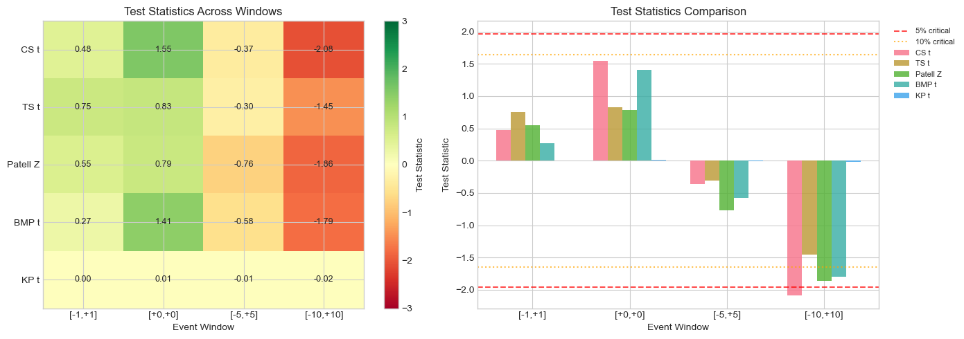
9. Power Analysis: Monte Carlo Simulation
Understanding Test Power
Power = Probability of rejecting when it is false
We want tests with:
Correct size (reject at stated significance level under )
High power (detect true effects)
Simulation Setup
Generate synthetic abnormal returns with known properties
Apply different tests
Measure rejection rates under (size) and (power)
Source
def simulate_event_study(N: int, T_est: int, L_event: int,
                         true_car: float = 0.0,
                         sigma: float = 0.02,
                         event_variance_multiplier: float = 1.0) -> List[Dict]:
    """
    Simulate event study data for power analysis.

    Parameters:
    -----------
    N : int
        Number of events
    T_est : int
        Estimation window length
    L_event : int
        Event window length
    true_car : float
        True cumulative abnormal return (0 under null)
    sigma : float
        Residual standard deviation
    event_variance_multiplier : float
        Multiplier for event window variance (>1 means event-induced variance)

    Returns:
    --------
    List of simulated event results
    """
    results = []

    # True abnormal return per day (spread evenly)
    true_ar_daily = true_car / L_event

    for i in range(N):
        # Generate estimation period residuals
        est_residuals = np.random.normal(0, sigma, T_est)

        # Generate event window abnormal returns
        event_sigma = sigma * np.sqrt(event_variance_multiplier)
        event_ar = np.random.normal(true_ar_daily, event_sigma, L_event)

        # Create mock model
        model = MarketModelResults(
            alpha=0.0,
            beta=1.0,
            sigma=np.std(est_residuals, ddof=2),
            r_squared=0.3,
            n_obs=T_est,
            market_mean=0.0005,
            market_var=T_est * 0.0001,
            residuals=est_residuals
        )

        # Create event data
        event_data = pd.DataFrame({
            'event_time': range(-L_event//2, L_event//2 + L_event%2),
            'stock_ret': event_ar + 0.0005,  # Add expected return
            'market_ret': np.random.normal(0.0005, 0.01, L_event),
            'expected_ret': np.full(L_event, 0.0005),
            'AR': event_ar
        })

        results.append({
            'model': model,
            'event_data': event_data
        })

    return results


def run_simulation_tests(sim_results: List[Dict], tau1: int, tau2: int) -> Dict:
    """
    Run all tests on simulated data.
    """
    # Convert to format expected by test functions
    class MockResult:
        def __init__(self, d):
            self.model = d['model']
            self.event_data = d['event_data']

    mock_results = [MockResult(d) for d in sim_results]

    cs = cross_sectional_t_test(mock_results, tau1, tau2)
    patell = patell_test(mock_results, tau1, tau2)
    bmp = bmp_test(mock_results, tau1, tau2)

    return {
        'CS_p': cs['p_value'],
        'Patell_p': patell['p_value'],
        'BMP_p': bmp['p_value']
    }


def monte_carlo_power(N_events: int, N_sims: int, true_car: float,
                      event_var_mult: float = 1.0,
                      alpha: float = 0.05) -> Dict:
    """
    Monte Carlo simulation for test power/size.
    """
    rejections = {'CS': 0, 'Patell': 0, 'BMP': 0}

    for _ in range(N_sims):
        sim_data = simulate_event_study(
            N=N_events, T_est=120, L_event=3,
            true_car=true_car, sigma=0.02,
            event_variance_multiplier=event_var_mult
        )

        results = run_simulation_tests(sim_data, -1, 1)

        if results['CS_p'] < alpha:
            rejections['CS'] += 1
        if results['Patell_p'] < alpha:
            rejections['Patell'] += 1
        if results['BMP_p'] < alpha:
            rejections['BMP'] += 1

    return {
        'CS_rejection_rate': rejections['CS'] / N_sims,
        'Patell_rejection_rate': rejections['Patell'] / N_sims,
        'BMP_rejection_rate': rejections['BMP'] / N_sims
    }


print("Monte Carlo Simulation: Test Size and Power")
print("="*70)
print("(This may take a moment...)\n")

N_SIMS = 500  # Reduced for speed; use 1000+ for research
N_EVENTS = 30

# Test size under H0 (true_car = 0)
print("1. SIZE (H0: CAR = 0, No event-induced variance)")
size_results = monte_carlo_power(N_EVENTS, N_SIMS, true_car=0.0, event_var_mult=1.0)
print(f"   CS t-test:    {size_results['CS_rejection_rate']*100:.1f}% (nominal: 5%)")
print(f"   Patell test:  {size_results['Patell_rejection_rate']*100:.1f}%")
print(f"   BMP test:     {size_results['BMP_rejection_rate']*100:.1f}%")

# Test size with event-induced variance
print("\n2. SIZE WITH EVENT-INDUCED VARIANCE (H0: CAR = 0, Variance x2)")
size_eiv = monte_carlo_power(N_EVENTS, N_SIMS, true_car=0.0, event_var_mult=2.0)
print(f"   CS t-test:    {size_eiv['CS_rejection_rate']*100:.1f}%")
print(f"   Patell test:  {size_eiv['Patell_rejection_rate']*100:.1f}% <- Over-rejects!")
print(f"   BMP test:     {size_eiv['BMP_rejection_rate']*100:.1f}% <- Robust")

# Test power
print("\n3. POWER (H1: CAR = 1%)")
power_results = monte_carlo_power(N_EVENTS, N_SIMS, true_car=0.01, event_var_mult=1.0)
print(f"   CS t-test:    {power_results['CS_rejection_rate']*100:.1f}%")
print(f"   Patell test:  {power_results['Patell_rejection_rate']*100:.1f}%")
print(f"   BMP test:     {power_results['BMP_rejection_rate']*100:.1f}%")
Monte Carlo Simulation: Test Size and Power
======================================================================
(This may take a moment...)
1. SIZE (H0: CAR = 0, No event-induced variance)
---------------------------------------------------------------------------
ValueError                                Traceback (most recent call last)
Cell In[31], line 132
    130 # Test size under H0 (true_car = 0)
    131 print("1. SIZE (H0: CAR = 0, No event-induced variance)")
--> 132 size_results = monte_carlo_power(N_EVENTS, N_SIMS, true_car=0.0, event_var_mult=1.0)
    133 print(f"   CS t-test:    {size_results['CS_rejection_rate']*100:.1f}% (nominal: 5%)")
    134 print(f"   Patell test:  {size_results['Patell_rejection_rate']*100:.1f}%")

Cell In[31], line 101, in monte_carlo_power(N_events, N_sims, true_car, event_var_mult, alpha)
     98 rejections = {'CS': 0, 'Patell': 0, 'BMP': 0}
    100 for _ in range(N_sims):
--> 101     sim_data = simulate_event_study(
    102         N=N_events, T_est=120, L_event=3,
    103         true_car=true_car, sigma=0.02,
    104         event_variance_multiplier=event_var_mult
    105     )
    107     results = run_simulation_tests(sim_data, -1, 1)
    109     if results['CS_p'] < alpha:

Cell In[31], line 53, in simulate_event_study(N, T_est, L_event, true_car, sigma, event_variance_multiplier)
     41     model = MarketModelResults(
     42         alpha=0.0,
     43         beta=1.0,
   (...)
     49         residuals=est_residuals
     50     )
     52     # Create event data
---> 53     event_data = pd.DataFrame({
     54         'event_time': range(-L_event//2, L_event//2 + L_event%2),
     55         'stock_ret': event_ar + 0.0005,  # Add expected return
     56         'market_ret': np.random.normal(0.0005, 0.01, L_event),
     57         'expected_ret': np.full(L_event, 0.0005),
     58         'AR': event_ar
     59     })
     61     results.append({
     62         'model': model,
     63         'event_data': event_data
     64     })
     66 return results

File ~\AppData\Local\anaconda3\Lib\site-packages\pandas\core\frame.py:778, in DataFrame.__init__(self, data, index, columns, dtype, copy)
    772     mgr = self._init_mgr(
    773         data, axes={"index": index, "columns": columns}, dtype=dtype, copy=copy
    774     )
    776 elif isinstance(data, dict):
    777     # GH#38939 de facto copy defaults to False only in non-dict cases
--> 778     mgr = dict_to_mgr(data, index, columns, dtype=dtype, copy=copy, typ=manager)
    779 elif isinstance(data, ma.MaskedArray):
    780     from numpy.ma import mrecords

File ~\AppData\Local\anaconda3\Lib\site-packages\pandas\core\internals\construction.py:503, in dict_to_mgr(data, index, columns, dtype, typ, copy)
    499     else:
    500         # dtype check to exclude e.g. range objects, scalars
    501         arrays = [x.copy() if hasattr(x, "dtype") else x for x in arrays]
--> 503 return arrays_to_mgr(arrays, columns, index, dtype=dtype, typ=typ, consolidate=copy)

File ~\AppData\Local\anaconda3\Lib\site-packages\pandas\core\internals\construction.py:114, in arrays_to_mgr(arrays, columns, index, dtype, verify_integrity, typ, consolidate)
    111 if verify_integrity:
    112     # figure out the index, if necessary
    113     if index is None:
--> 114         index = _extract_index(arrays)
    115     else:
    116         index = ensure_index(index)

File ~\AppData\Local\anaconda3\Lib\site-packages\pandas\core\internals\construction.py:677, in _extract_index(data)
    675 lengths = list(set(raw_lengths))
    676 if len(lengths) > 1:
--> 677     raise ValueError("All arrays must be of the same length")
    679 if have_dicts:
    680     raise ValueError(
    681         "Mixing dicts with non-Series may lead to ambiguous ordering."
    682     )

ValueError: All arrays must be of the same length
Source
# Power curve as function of true CAR
print("\nGenerating power curves (this may take a minute)...")

true_cars = [0, 0.005, 0.01, 0.015, 0.02, 0.025, 0.03]
power_data = {'CAR': [], 'CS': [], 'Patell': [], 'BMP': []}

for car in true_cars:
    result = monte_carlo_power(N_EVENTS, 300, true_car=car)
    power_data['CAR'].append(car * 100)
    power_data['CS'].append(result['CS_rejection_rate'] * 100)
    power_data['Patell'].append(result['Patell_rejection_rate'] * 100)
    power_data['BMP'].append(result['BMP_rejection_rate'] * 100)
    print(f"  CAR = {car*100:.1f}%: CS={result['CS_rejection_rate']*100:.0f}%, "
          f"Patell={result['Patell_rejection_rate']*100:.0f}%, "
          f"BMP={result['BMP_rejection_rate']*100:.0f}%")

# Plot power curves
fig, ax = plt.subplots(figsize=(10, 6))

ax.plot(power_data['CAR'], power_data['CS'], 'b-o', label='CS t-test', markersize=8)
ax.plot(power_data['CAR'], power_data['Patell'], 'g-s', label='Patell', markersize=8)
ax.plot(power_data['CAR'], power_data['BMP'], 'r-^', label='BMP', markersize=8)

ax.axhline(5, color='gray', linestyle='--', alpha=0.7, label='5% significance')
ax.axhline(80, color='gray', linestyle=':', alpha=0.7, label='80% power target')

ax.set_xlabel('True CAR (%)', fontsize=12)
ax.set_ylabel('Rejection Rate (%)', fontsize=12)
ax.set_title(f'Power Curves (N={N_EVENTS} events, 5% significance)', fontsize=14)
ax.legend()
ax.grid(True, alpha=0.3)
ax.set_ylim(0, 100)

plt.tight_layout()
plt.show()
Generating power curves (this may take a minute)...
---------------------------------------------------------------------------
ValueError                                Traceback (most recent call last)
Cell In[33], line 8
      5 power_data = {'CAR': [], 'CS': [], 'Patell': [], 'BMP': []}
      7 for car in true_cars:
----> 8     result = monte_carlo_power(N_EVENTS, 300, true_car=car)
      9     power_data['CAR'].append(car * 100)
     10     power_data['CS'].append(result['CS_rejection_rate'] * 100)

Cell In[31], line 101, in monte_carlo_power(N_events, N_sims, true_car, event_var_mult, alpha)
     98 rejections = {'CS': 0, 'Patell': 0, 'BMP': 0}
    100 for _ in range(N_sims):
--> 101     sim_data = simulate_event_study(
    102         N=N_events, T_est=120, L_event=3,
    103         true_car=true_car, sigma=0.02,
    104         event_variance_multiplier=event_var_mult
    105     )
    107     results = run_simulation_tests(sim_data, -1, 1)
    109     if results['CS_p'] < alpha:

Cell In[31], line 53, in simulate_event_study(N, T_est, L_event, true_car, sigma, event_variance_multiplier)
     41     model = MarketModelResults(
     42         alpha=0.0,
     43         beta=1.0,
   (...)
     49         residuals=est_residuals
     50     )
     52     # Create event data
---> 53     event_data = pd.DataFrame({
     54         'event_time': range(-L_event//2, L_event//2 + L_event%2),
     55         'stock_ret': event_ar + 0.0005,  # Add expected return
     56         'market_ret': np.random.normal(0.0005, 0.01, L_event),
     57         'expected_ret': np.full(L_event, 0.0005),
     58         'AR': event_ar
     59     })
     61     results.append({
     62         'model': model,
     63         'event_data': event_data
     64     })
     66 return results

File ~\AppData\Local\anaconda3\Lib\site-packages\pandas\core\frame.py:778, in DataFrame.__init__(self, data, index, columns, dtype, copy)
    772     mgr = self._init_mgr(
    773         data, axes={"index": index, "columns": columns}, dtype=dtype, copy=copy
    774     )
    776 elif isinstance(data, dict):
    777     # GH#38939 de facto copy defaults to False only in non-dict cases
--> 778     mgr = dict_to_mgr(data, index, columns, dtype=dtype, copy=copy, typ=manager)
    779 elif isinstance(data, ma.MaskedArray):
    780     from numpy.ma import mrecords

File ~\AppData\Local\anaconda3\Lib\site-packages\pandas\core\internals\construction.py:503, in dict_to_mgr(data, index, columns, dtype, typ, copy)
    499     else:
    500         # dtype check to exclude e.g. range objects, scalars
    501         arrays = [x.copy() if hasattr(x, "dtype") else x for x in arrays]
--> 503 return arrays_to_mgr(arrays, columns, index, dtype=dtype, typ=typ, consolidate=copy)

File ~\AppData\Local\anaconda3\Lib\site-packages\pandas\core\internals\construction.py:114, in arrays_to_mgr(arrays, columns, index, dtype, verify_integrity, typ, consolidate)
    111 if verify_integrity:
    112     # figure out the index, if necessary
    113     if index is None:
--> 114         index = _extract_index(arrays)
    115     else:
    116         index = ensure_index(index)

File ~\AppData\Local\anaconda3\Lib\site-packages\pandas\core\internals\construction.py:677, in _extract_index(data)
    675 lengths = list(set(raw_lengths))
    676 if len(lengths) > 1:
--> 677     raise ValueError("All arrays must be of the same length")
    679 if have_dicts:
    680     raise ValueError(
    681         "Mixing dicts with non-Series may lead to ambiguous ordering."
    682     )

ValueError: All arrays must be of the same length
10. Practical Guidelines
Which Test to Use?
| Situation | Recommended Test | Reason |
|---|---|---|
| General use | BMP | Robust to event-induced variance |
| No event clustering | Patell | More powerful when assumptions hold |
| Event clustering | Kolari-Pynnönen | Adjusts for cross-correlation |
| Very small sample (N<10) | Cross-sectional t | Simple, interpretable |
| Heterogeneous firms | BMP or KP | Account for variance differences |
Reporting Best Practices
Report multiple tests for robustness
Include both CAAR and test statistics
Note sample size and any clustering
Report results for multiple windows
Discuss economic vs. statistical significance
Source
def create_publication_table(event_results: List[EventStudyResult],
                              windows: List[Tuple[int, int]]) -> pd.DataFrame:
    """
    Create a publication-ready results table.
    """
    rows = []

    for tau1, tau2 in windows:
        cars = [calculate_car(r.event_data, tau1, tau2) for r in event_results]
        caar = np.mean(cars)

        cs = cross_sectional_t_test(event_results, tau1, tau2)
        patell = patell_test(event_results, tau1, tau2)
        bmp = bmp_test(event_results, tau1, tau2)

        def sig(p):
            if p < 0.01: return '***'
            elif p < 0.05: return '**'
            elif p < 0.10: return '*'
            return ''

        rows.append({
            'Window': f'[{tau1:+d}, {tau2:+d}]',
            'N': len(event_results),
            'CAAR (%)': f"{caar*100:+.2f}",
            'CS t-stat': f"{cs['t_stat']:.2f}{sig(cs['p_value'])}",
            'Patell Z': f"{patell['Z_stat']:.2f}{sig(patell['p_value'])}",
            'BMP t-stat': f"{bmp['t_stat']:.2f}{sig(bmp['p_value'])}"
        })

    return pd.DataFrame(rows)


# Generate publication table
print("\n" + "="*90)
print("PUBLICATION-READY RESULTS TABLE")
print("="*90)
print("\nTable: Cumulative Average Abnormal Returns Around Earnings Announcements")
print("Sample: Tech companies, Q2-Q3 2023 earnings")
print("-"*90)

pub_table = create_publication_table(event_results, windows)
print(pub_table.to_string(index=False))

print("-"*90)
print("Notes: ***, **, * indicate significance at 1%, 5%, 10% levels.")
print("CS = cross-sectional t-test; Patell = Patell (1976) standardized test;")
print("BMP = Boehmer et al. (1991) standardized cross-sectional test.")
==========================================================================================
PUBLICATION-READY RESULTS TABLE
==========================================================================================

Table: Cumulative Average Abnormal Returns Around Earnings Announcements
Sample: Tech companies, Q2-Q3 2023 earnings
------------------------------------------------------------------------------------------
    Window  N CAAR (%) CS t-stat Patell Z BMP t-stat
  [-1, +1] 10    +0.96      0.48     0.55       0.27
  [+0, +0] 10    +0.60      1.55     0.79       1.41
  [-5, +5] 10    -0.76     -0.37    -0.76      -0.58
[-10, +10] 10    -5.23    -2.08*   -1.86*      -1.79
------------------------------------------------------------------------------------------
Notes: ***, **, * indicate significance at 1%, 5%, 10% levels.
CS = cross-sectional t-test; Patell = Patell (1976) standardized test;
BMP = Boehmer et al. (1991) standardized cross-sectional test.
11. Exercises
Exercise 1: Sample Size Sensitivity
Using Monte Carlo simulation, examine how test power changes with sample size (N = 10, 30, 50, 100).
Exercise 2: Window Length Effects
How does test power change as you lengthen the event window? Why?
Exercise 3: Skewness Adjustment
Implement a skewness-adjusted t-test that accounts for non-normality in CARs.
Exercise 4: Calendar-Time Portfolio
Implement a calendar-time portfolio approach that forms portfolios of event firms and regresses on market factors.
Source
# Exercise 3 Template: Skewness-Adjusted t-Test

def skewness_adjusted_t_test(event_results: List[EventStudyResult],
                              tau1: int, tau2: int) -> Dict:
    """
    Hall (1992) skewness-adjusted t-test.

    Adjusts for skewness in the CAR distribution.
    """
    cars = np.array([calculate_car(r.event_data, tau1, tau2) for r in event_results])
    N = len(cars)

    # Standard t-test components
    mean_car = np.mean(cars)
    std_car = np.std(cars, ddof=1)
    se = std_car / np.sqrt(N)
    t_standard = mean_car / se if se > 0 else 0

    # Skewness
    skew = stats.skew(cars)

    # Hall (1992) adjustment
    # t_adj = t + (1/6) * skew * (t^2 + 2) / sqrt(N)
    t_adjusted = t_standard + (1/6) * skew * (t_standard**2 + 2) / np.sqrt(N)

    p_value = 2 * (1 - stats.t.cdf(abs(t_adjusted), df=N-1))

    return {
        'test_name': 'Skewness-Adjusted t',
        'N': N,
        'CAAR': mean_car,
        'skewness': skew,
        't_standard': t_standard,
        't_adjusted': t_adjusted,
        'p_value': p_value
    }


# Test the skewness-adjusted t-test
print("Skewness-Adjusted t-Test:")
print("="*50)

for tau1, tau2 in [(-1, +1), (0, 0)]:
    result = skewness_adjusted_t_test(event_results, tau1, tau2)
    print(f"\nWindow [{tau1:+d}, {tau2:+d}]:")
    print(f"  Skewness = {result['skewness']:.3f}")
    print(f"  Standard t = {result['t_standard']:.3f}")
    print(f"  Adjusted t = {result['t_adjusted']:.3f}")
    print(f"  p-value = {result['p_value']:.4f}")
Skewness-Adjusted t-Test:
==================================================
Window [-1, +1]:
Skewness = -0.507
Standard t = 0.475
Adjusted t = 0.416
p-value = 0.6873
Window [+0, +0]:
Skewness = -0.001
Standard t = 1.550
Adjusted t = 1.550
p-value = 0.1556
12. Summary
In this session, we covered:
Cross-Sectional t-Test: Simple but assumes homogeneous variance
Time-Series t-Test: Uses estimation period variance
Patell (1976) Test: Standardizes ARs, more powerful but assumes no event-induced variance
BMP (1991) Test: Robust to event-induced variance changes
Kolari-Pynnönen (2010): Adjusts for cross-correlation
Monte Carlo Analysis: Understanding test size and power
Key Takeaways
BMP is the recommended default for most applications
Event-induced variance is common and Patell over-rejects
Cross-correlation from event clustering requires adjustment
Report multiple tests for robustness
Consider economic significance alongside statistical significance
Coming Up Next
Session 5: Statistical Inference II - Non-Parametric and Robust Tests will cover:
Sign test and generalized sign test
Rank tests (Corrado, Corrado-Zivney)
Bootstrap methods
Dealing with non-normality
13. References
Core Methodology
Patell, J. M. (1976). Corporate forecasts of earnings per share and stock price behavior. Journal of Accounting Research, 14(2), 246-276.
Boehmer, E., Musumeci, J., & Poulsen, A. B. (1991). Event-study methodology under conditions of event-induced variance. Journal of Financial Economics, 30(2), 253-272.
Kolari, J. W., & Pynnönen, S. (2010). Event study testing with cross-sectional correlation of abnormal returns. Review of Financial Studies, 23(11), 3996-4025.
Power and Specification
Brown, S. J., & Warner, J. B. (1985). Using daily stock returns: The case of event studies. Journal of Financial Economics, 14(1), 3-31.
Campbell, J. Y., Lo, A. W., & MacKinlay, A. C. (1997). The Econometrics of Financial Markets. Princeton University Press.