Session 3: Asymmetric GARCH Models
Course: Advanced Volatility Modeling
Learning Objectives
By the end of this session, students will be able to:
Understand the leverage effect and its economic interpretation
Derive and estimate EGARCH, GJR-GARCH, and TGARCH models
Compare news impact curves across models
Test for asymmetry in volatility response
1. The Leverage Effect
1.1 Empirical Evidence
Black (1976) documented that stock returns and volatility are negatively correlated:
Negative returns → Increased future volatility
Positive returns → Decreased (or unchanged) future volatility
This asymmetry is called the leverage effect.
1.2 Economic Explanations
Leverage hypothesis (Black, 1976; Christie, 1982):
When stock price falls, debt-to-equity ratio rises
Higher leverage → higher risk → higher volatility
Volatility feedback hypothesis (French et al., 1987; Campbell & Hentschel, 1992):
News of higher future volatility raises required return
Stock price must fall immediately to deliver higher expected return
1.3 News Impact Curve
The News Impact Curve (NIC) shows how today’s shock affects tomorrow’s variance:
For symmetric GARCH(1,1), the NIC is a parabola centered at zero.
Source
import numpy as np
import pandas as pd
import matplotlib.pyplot as plt
import scipy.stats as stats
from scipy.optimize import minimize
import yfinance as yf
from arch import arch_model
import warnings
warnings.filterwarnings('ignore')

plt.style.use('seaborn-v0_8-whitegrid')
plt.rcParams['figure.figsize'] = (12, 6)
plt.rcParams['font.size'] = 11

np.random.seed(42)
Source
# Download S&P 500 data
spy = yf.download('SPY', start='2010-01-01', end='2024-12-31', progress=False)
if isinstance(spy.columns, pd.MultiIndex):
    spy.columns = spy.columns.get_level_values(0)

spy['returns'] = np.log(spy['Close'] / spy['Close'].shift(1))
returns = spy['returns'].dropna() * 100  # Percentage returns

print(f"Sample: {returns.index[0].date()} to {returns.index[-1].date()}")
print(f"Observations: {len(returns)}")
YF.download() has changed argument auto_adjust default to True
Sample: 2010-01-05 to 2024-12-30
Observations: 3772
Source
# Empirical evidence of leverage effect
def empirical_leverage_effect(returns, lags=20):
    """
    Compute cross-correlation between returns and future squared returns.
    Leverage effect implies negative correlation at positive lags.
    """
    ret = returns - returns.mean()
    sq_ret = ret ** 2

    correlations = []
    for lag in range(-lags, lags + 1):
        if lag < 0:
            corr = ret.iloc[-lag:].corr(sq_ret.iloc[:lag])
        elif lag > 0:
            corr = ret.iloc[:-lag].corr(sq_ret.iloc[lag:])
        else:
            corr = ret.corr(sq_ret)
        correlations.append(corr)

    return np.arange(-lags, lags + 1), np.array(correlations)

lags, corrs = empirical_leverage_effect(returns)

fig, ax = plt.subplots(figsize=(12, 5))
colors = ['green' if c > 0 else 'red' for c in corrs]
ax.bar(lags, corrs, color=colors, alpha=0.7, edgecolor='white')
ax.axhline(0, color='black', linewidth=0.5)
ax.axvline(0, color='black', linewidth=0.5, linestyle='--')
ax.set_xlabel('Lag k')
ax.set_ylabel('Corr(r_t, r²_{t+k})')
ax.set_title('S&P 500: Cross-Correlation of Returns with Future Squared Returns', fontsize=13)

plt.tight_layout()
plt.show()

print(f"\nCorr(r_t, r²_{{t+1}}): {corrs[lags==1][0]:.4f}")
print(f"Corr(r_t, r²_{{t+5}}): {corrs[lags==5][0]:.4f}")
print("\nNegative values at positive lags confirm the leverage effect.")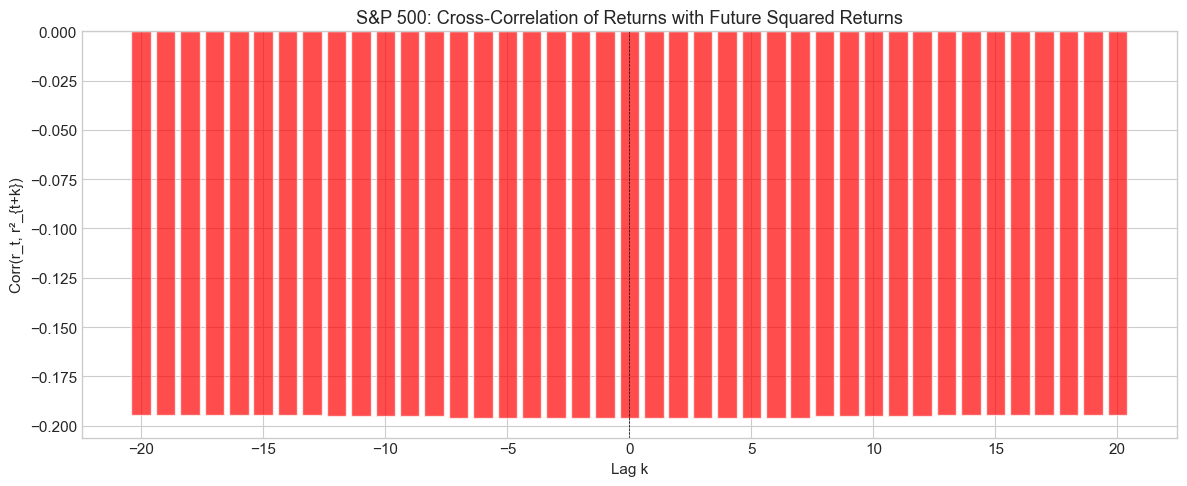
Corr(r_t, r²_{t+1}): -0.1962
Corr(r_t, r²_{t+5}): -0.1962

Negative values at positive lags confirm the leverage effect.
2. GJR-GARCH (Glosten-Jagannathan-Runkle)
2.1 Model Specification
GJR-GARCH(1,1) adds an asymmetric term for negative shocks:
where is an indicator for negative shocks.
Interpretation:
Positive shock (): Impact is
Negative shock (): Impact is
indicates leverage effect
2.2 Stationarity Condition
2.3 News Impact Curve
Source
def simulate_gjr_garch(n, omega, alpha, gamma, beta, dist='normal', df=5):
    """
    Simulate GJR-GARCH(1,1) process.
    """
    eps = np.zeros(n)
    sigma2 = np.zeros(n)

    if dist == 'normal':
        z = np.random.standard_normal(n)
    else:
        z = np.random.standard_t(df, n) / np.sqrt(df / (df - 2))

    uncond_var = omega / (1 - alpha - gamma/2 - beta)
    sigma2[0] = uncond_var
    eps[0] = np.sqrt(sigma2[0]) * z[0]

    for t in range(1, n):
        indicator = 1 if eps[t-1] < 0 else 0
        sigma2[t] = omega + alpha * eps[t-1]**2 + gamma * eps[t-1]**2 * indicator + beta * sigma2[t-1]
        eps[t] = np.sqrt(sigma2[t]) * z[t]

    return eps, sigma2

# Simulate GJR-GARCH
n = 2000
omega, alpha, gamma, beta = 0.05, 0.05, 0.10, 0.85

np.random.seed(42)
eps_gjr, sigma2_gjr = simulate_gjr_garch(n, omega, alpha, gamma, beta)

fig, axes = plt.subplots(2, 1, figsize=(14, 8))

axes[0].plot(eps_gjr, color='steelblue', linewidth=0.5)
axes[0].set_title('Simulated GJR-GARCH(1,1) Returns', fontsize=12)
axes[0].set_ylabel('Returns')

axes[1].plot(np.sqrt(sigma2_gjr), color='red', linewidth=0.8)
axes[1].set_title('Conditional Volatility', fontsize=12)
axes[1].set_ylabel('σ_t')

plt.tight_layout()
plt.show()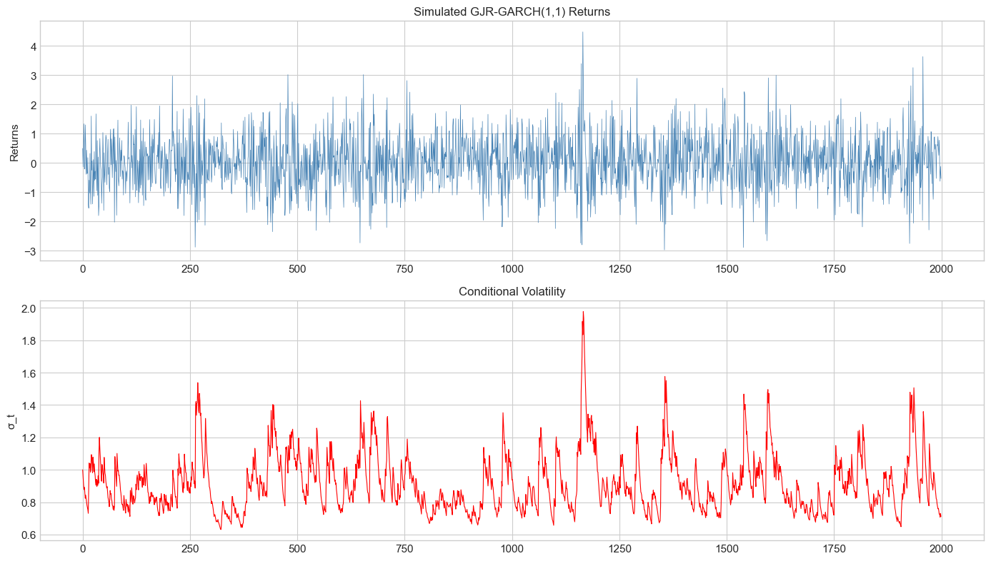
Source
# Fit GJR-GARCH to S&P 500
model_gjr = arch_model(returns, vol='Garch', p=1, o=1, q=1, dist='t')
fit_gjr = model_gjr.fit(disp='off')

print("GJR-GARCH(1,1) Estimation Results")
print("="*60)
print(fit_gjr.summary())

alpha_hat = fit_gjr.params['alpha[1]']
gamma_hat = fit_gjr.params['gamma[1]']

print(f"\n\nInterpretation:")
print(f"Impact of positive shock: α = {alpha_hat:.4f}")
print(f"Impact of negative shock: α + γ = {alpha_hat + gamma_hat:.4f}")
print(f"Asymmetry ratio: (α + γ)/α = {(alpha_hat + gamma_hat)/max(alpha_hat, 0.001):.2f}")
GJR-GARCH(1,1) Estimation Results
============================================================
Constant Mean - GJR-GARCH Model Results
====================================================================================
Dep. Variable: returns R-squared: 0.000
Mean Model: Constant Mean Adj. R-squared: 0.000
Vol Model: GJR-GARCH Log-Likelihood: -4643.32
Distribution: Standardized Student's t AIC: 9298.65
Method: Maximum Likelihood BIC: 9336.06
No. Observations: 3772
Date: Thu, Feb 05 2026 Df Residuals: 3771
Time: 09:32:08 Df Model: 1
Mean Model
============================================================================
coef std err t P>|t| 95.0% Conf. Int.
----------------------------------------------------------------------------
mu 0.0747 1.054e-02 7.091 1.334e-12 [5.406e-02,9.536e-02]
Volatility Model
=============================================================================
coef std err t P>|t| 95.0% Conf. Int.
-----------------------------------------------------------------------------
omega 0.0288 4.634e-03 6.223 4.885e-10 [1.976e-02,3.792e-02]
alpha[1] 2.0125e-12 1.317e-02 1.529e-10 1.000 [-2.580e-02,2.580e-02]
gamma[1] 0.2917 3.587e-02 8.131 4.244e-16 [ 0.221, 0.362]
beta[1] 0.8303 1.690e-02 49.133 0.000 [ 0.797, 0.863]
Distribution
========================================================================
coef std err t P>|t| 95.0% Conf. Int.
------------------------------------------------------------------------
nu 5.8145 0.566 10.264 1.024e-24 [ 4.704, 6.925]
========================================================================
Covariance estimator: robust
Interpretation:
Impact of positive shock: α = 0.0000
Impact of negative shock: α + γ = 0.2917
Asymmetry ratio: (α + γ)/α = 291.69
3. EGARCH (Exponential GARCH)
3.1 Model Specification
Nelson (1991) proposed EGARCH, which models log-variance:
where and:
3.2 Key Properties
Advantages over GJR-GARCH:
No parameter restrictions for positivity (since we model log-variance)
Continuous news impact curve at zero
Log-linear structure facilitates interpretation
Asymmetry: implies leverage effect
Source
# Fit EGARCH to S&P 500
model_egarch = arch_model(returns, vol='EGARCH', p=1, o=1, q=1, dist='t')
fit_egarch = model_egarch.fit(disp='off')

print("EGARCH(1,1) Estimation Results")
print("="*60)
print(fit_egarch.summary())

print(f"\n\nNote: In EGARCH, alpha[1] < 0 indicates leverage effect.")
print(f"alpha[1] = {fit_egarch.params['alpha[1]']:.4f}")
EGARCH(1,1) Estimation Results
============================================================
Constant Mean - EGARCH Model Results
====================================================================================
Dep. Variable: returns R-squared: 0.000
Mean Model: Constant Mean Adj. R-squared: 0.000
Vol Model: EGARCH Log-Likelihood: -4630.50
Distribution: Standardized Student's t AIC: 9273.01
Method: Maximum Likelihood BIC: 9310.42
No. Observations: 3772
Date: Thu, Feb 05 2026 Df Residuals: 3771
Time: 09:32:20 Df Model: 1
Mean Model
============================================================================
coef std err t P>|t| 95.0% Conf. Int.
----------------------------------------------------------------------------
mu 0.0694 1.062e-02 6.532 6.508e-11 [4.855e-02,9.018e-02]
Volatility Model
==============================================================================
coef std err t P>|t| 95.0% Conf. Int.
------------------------------------------------------------------------------
omega -9.4307e-03 5.012e-03 -1.882 5.987e-02 [-1.925e-02,3.919e-04]
alpha[1] 0.1876 2.126e-02 8.823 1.115e-18 [ 0.146, 0.229]
gamma[1] -0.1973 1.610e-02 -12.257 1.534e-34 [ -0.229, -0.166]
beta[1] 0.9642 6.178e-03 156.062 0.000 [ 0.952, 0.976]
Distribution
========================================================================
coef std err t P>|t| 95.0% Conf. Int.
------------------------------------------------------------------------
nu 6.0058 0.601 9.989 1.697e-23 [ 4.827, 7.184]
========================================================================
Covariance estimator: robust
Note: In EGARCH, alpha[1] < 0 indicates leverage effect.
alpha[1] = 0.1876
4. News Impact Curves Comparison
Source
# Fit symmetric GARCH for comparison
model_garch = arch_model(returns, vol='Garch', p=1, q=1, dist='t')
fit_garch = model_garch.fit(disp='off')

def compute_news_impact_curve(fit, model_type, shock_range, uncond_var):
    """Compute news impact curve for a given model."""
    params = fit.params
    sample_std = np.sqrt(uncond_var)
    shocks = shock_range * sample_std

    if model_type == 'GARCH':
        omega = params['omega']
        alpha = params['alpha[1]']
        beta = params['beta[1]']
        nic = omega + beta * uncond_var + alpha * shocks**2

    elif model_type == 'GJR':
        omega = params['omega']
        alpha = params['alpha[1]']
        gamma = params['gamma[1]']
        beta = params['beta[1]']
        nic = omega + beta * uncond_var + alpha * shocks**2
        nic[shocks < 0] += gamma * shocks[shocks < 0]**2

    elif model_type == 'EGARCH':
        omega = params['omega']
        alpha = params['alpha[1]']
        gamma = params['gamma[1]']
        beta = params['beta[1]']
        z = shocks / sample_std
        log_var = omega + beta * np.log(uncond_var) + alpha * z + gamma * (np.abs(z) - np.sqrt(2/np.pi))
        nic = np.exp(log_var)

    return shocks, nic

# Compute NICs
shock_range = np.linspace(-4, 4, 200)
uncond_var = returns.var()

shocks_g, nic_garch = compute_news_impact_curve(fit_garch, 'GARCH', shock_range, uncond_var)
shocks_j, nic_gjr = compute_news_impact_curve(fit_gjr, 'GJR', shock_range, uncond_var)
shocks_e, nic_egarch = compute_news_impact_curve(fit_egarch, 'EGARCH', shock_range, uncond_var)

# Plot
fig, ax = plt.subplots(figsize=(12, 7))

ax.plot(shocks_g, np.sqrt(nic_garch), 'b-', linewidth=2, label='GARCH(1,1)')
ax.plot(shocks_j, np.sqrt(nic_gjr), 'r--', linewidth=2, label='GJR-GARCH(1,1)')
ax.plot(shocks_e, np.sqrt(nic_egarch), 'g-.', linewidth=2, label='EGARCH(1,1)')

ax.axvline(0, color='gray', linestyle=':', alpha=0.5)
ax.set_xlabel('Shock ε_{t-1}', fontsize=12)
ax.set_ylabel('Conditional Volatility σ_t', fontsize=12)
ax.set_title('News Impact Curves: Symmetric vs Asymmetric Models', fontsize=14)
ax.legend(loc='upper center', fontsize=11)

plt.tight_layout()
plt.show()

print("\nKey observations:")
print("1. GARCH is symmetric (parabola centered at zero)")
print("2. GJR-GARCH has a kink at zero - steeper on the left (negative shocks)")
print("3. EGARCH is smooth and asymmetric")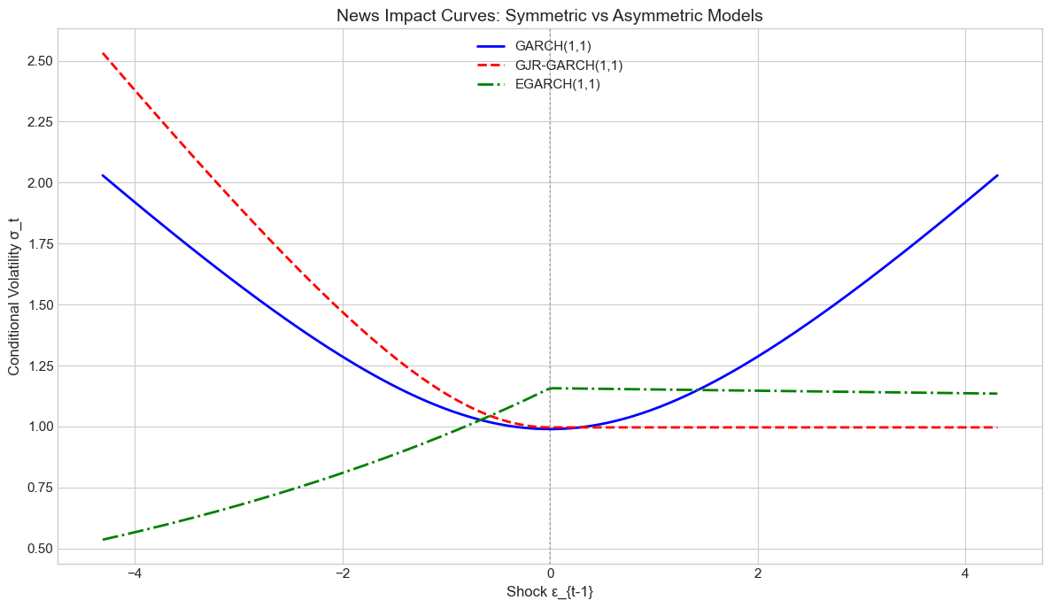
Key observations:
1. GARCH is symmetric (parabola centered at zero)
2. GJR-GARCH has a kink at zero - steeper on the left (negative shocks)
3. EGARCH is smooth and asymmetric
5. Testing for Asymmetry
5.1 Sign Bias Test (Engle & Ng, 1993)
Regress squared standardized residuals on sign indicators:
where and .
Sign bias test:
Negative size bias test:
Positive size bias test:
Joint test:
Source
import statsmodels.api as sm

def sign_bias_test(fitted_model):
    """
    Perform Engle-Ng sign bias tests for asymmetry.
    """
    std_resid = fitted_model.std_resid
    resid = fitted_model.resid

    # Create variables
    z2 = std_resid ** 2
    S_neg = (resid < 0).astype(float)
    S_pos = 1 - S_neg

    # Lag the indicators
    df = pd.DataFrame({
        'z2': z2,
        'S_neg_lag': S_neg.shift(1),
        'neg_size': S_neg.shift(1) * resid.shift(1),
        'pos_size': S_pos.shift(1) * resid.shift(1)
    }).dropna()

    # Regression
    X = sm.add_constant(df[['S_neg_lag', 'neg_size', 'pos_size']])
    y = df['z2']

    model = sm.OLS(y, X).fit()

    # Individual tests
    print("Engle-Ng Sign Bias Tests")
    print("="*60)
    print(f"\n{'Test':<25} {'Coef':>10} {'t-stat':>10} {'p-value':>10}")
    print("-"*60)

    tests = [
        ('Sign Bias', 'S_neg_lag'),
        ('Negative Size Bias', 'neg_size'),
        ('Positive Size Bias', 'pos_size')
    ]

    for test_name, var in tests:
        coef = model.params[var]
        tstat = model.tvalues[var]
        pval = model.pvalues[var]
        sig = '***' if pval < 0.01 else ('**' if pval < 0.05 else ('*' if pval < 0.1 else ''))
        print(f"{test_name:<25} {coef:>10.4f} {tstat:>10.2f} {pval:>10.4f} {sig}")

    # Joint test (F-test)
    r_matrix = np.eye(4)[1:]  # Test all except constant
    f_test = model.f_test(r_matrix)
    print(f"\n{'Joint Test':<25} {'F-stat':>10} {'':>10} {'p-value':>10}")
    print("-"*60)
    print(f"{'H0: c1=c2=c3=0':<25} {f_test.fvalue:>10.2f} {'':<10} {f_test.pvalue:>10.4f}")

    return model

# Test on symmetric GARCH residuals
print("Testing GARCH(1,1) residuals for asymmetry:")
sb_garch = sign_bias_test(fit_garch)

print("\n" + "="*60)
print("\nTesting GJR-GARCH(1,1) residuals for remaining asymmetry:")
sb_gjr = sign_bias_test(fit_gjr)
Testing GARCH(1,1) residuals for asymmetry:
Engle-Ng Sign Bias Tests
============================================================
Test Coef t-stat p-value
------------------------------------------------------------
Sign Bias 0.3460 3.88 0.0001 ***
Negative Size Bias 0.0629 1.20 0.2287
Positive Size Bias -0.0678 -1.03 0.3045
Joint Test F-stat p-value
------------------------------------------------------------
H0: c1=c2=c3=0 9.98 0.0000
============================================================
Testing GJR-GARCH(1,1) residuals for remaining asymmetry:
Engle-Ng Sign Bias Tests
============================================================
Test Coef t-stat p-value
------------------------------------------------------------
Sign Bias 0.3186 3.13 0.0018 ***
Negative Size Bias 0.1583 2.62 0.0089 ***
Positive Size Bias -0.0147 -0.20 0.8436
Joint Test F-stat p-value
------------------------------------------------------------
H0: c1=c2=c3=0 4.94 0.0020
6. Model Comparison
Source
# Compare all models
models = {
    'GARCH(1,1)': fit_garch,
    'GJR-GARCH(1,1)': fit_gjr,
    'EGARCH(1,1)': fit_egarch
}

comparison = []
for name, fit in models.items():
    comparison.append({
        'Model': name,
        'Log-Lik': fit.loglikelihood,
        'AIC': fit.aic,
        'BIC': fit.bic,
        'Params': fit.num_params
    })

comparison_df = pd.DataFrame(comparison).set_index('Model')
print("Model Comparison")
print("="*60)
print(comparison_df.round(2))
print(f"\nBest model by BIC: {comparison_df['BIC'].idxmin()}")
Model Comparison
============================================================
Log-Lik AIC BIC Params
Model
GARCH(1,1) -4711.96 9433.91 9465.09 5
GJR-GARCH(1,1) -4643.32 9298.65 9336.06 6
EGARCH(1,1) -4630.50 9273.01 9310.42 6
Best model by BIC: EGARCH(1,1)
Source
# Plot conditional volatility comparison
fig, axes = plt.subplots(3, 1, figsize=(14, 10), sharex=True)

for ax, (name, fit) in zip(axes, models.items()):
    vol = fit.conditional_volatility
    ax.plot(vol.index, vol.values, linewidth=0.8, label=name)
    ax.fill_between(vol.index, 0, vol.values, alpha=0.3)
    ax.set_ylabel('Volatility (%)')
    ax.set_title(name, fontsize=12)
    ax.set_ylim(0, vol.max() * 1.1)

plt.xlabel('Date')
plt.tight_layout()
plt.suptitle('Conditional Volatility: Model Comparison', y=1.01, fontsize=14, fontweight='bold')
plt.show()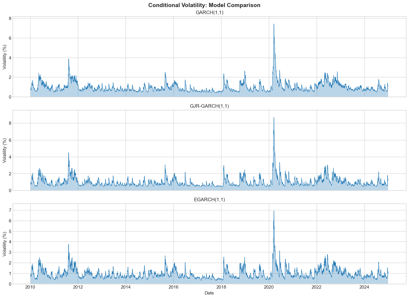
7. Cryptocurrency Application
Does the leverage effect exist in cryptocurrency markets?
Source
# Download Bitcoin data
btc = yf.download('BTC-USD', start='2018-01-01', end='2024-12-31', progress=False)
if isinstance(btc.columns, pd.MultiIndex):
    btc.columns = btc.columns.get_level_values(0)

btc_returns = (np.log(btc['Close'] / btc['Close'].shift(1)) * 100).dropna()

# Fit models
btc_garch = arch_model(btc_returns, vol='Garch', p=1, q=1, dist='t').fit(disp='off')
btc_gjr = arch_model(btc_returns, vol='Garch', p=1, o=1, q=1, dist='t').fit(disp='off')

print("Bitcoin: GARCH(1,1)")
print(btc_garch.summary())

print("\n\nBitcoin: GJR-GARCH(1,1)")
print(btc_gjr.summary())

btc_gamma = btc_gjr.params['gamma[1]']
print(f"\n\nBitcoin asymmetry parameter γ = {btc_gamma:.4f}")
if btc_gamma > 0:
    print("Bitcoin shows leverage effect (surprising for crypto!)")
else:
    print("Bitcoin shows inverse leverage effect (common in crypto)")
Bitcoin: GARCH(1,1)
Constant Mean - GARCH Model Results
====================================================================================
Dep. Variable: Close R-squared: 0.000
Mean Model: Constant Mean Adj. R-squared: 0.000
Vol Model: GARCH Log-Likelihood: -6402.25
Distribution: Standardized Student's t AIC: 12814.5
Method: Maximum Likelihood BIC: 12843.7
No. Observations: 2555
Date: Thu, Feb 05 2026 Df Residuals: 2554
Time: 09:35:05 Df Model: 1
Mean Model
===========================================================================
coef std err t P>|t| 95.0% Conf. Int.
---------------------------------------------------------------------------
mu 0.0740 4.189e-02 1.767 7.718e-02 [-8.071e-03, 0.156]
Volatility Model
============================================================================
coef std err t P>|t| 95.0% Conf. Int.
----------------------------------------------------------------------------
omega 0.1355 8.336e-02 1.626 0.104 [-2.784e-02, 0.299]
alpha[1] 0.0723 1.091e-02 6.627 3.436e-11 [5.091e-02,9.368e-02]
beta[1] 0.9277 1.334e-02 69.522 0.000 [ 0.902, 0.954]
Distribution
========================================================================
coef std err t P>|t| 95.0% Conf. Int.
------------------------------------------------------------------------
nu 3.1152 0.155 20.057 1.755e-89 [ 2.811, 3.420]
========================================================================
Covariance estimator: robust
Bitcoin: GJR-GARCH(1,1)
Constant Mean - GJR-GARCH Model Results
====================================================================================
Dep. Variable: Close R-squared: 0.000
Mean Model: Constant Mean Adj. R-squared: 0.000
Vol Model: GJR-GARCH Log-Likelihood: -6402.20
Distribution: Standardized Student's t AIC: 12816.4
Method: Maximum Likelihood BIC: 12851.5
No. Observations: 2555
Date: Thu, Feb 05 2026 Df Residuals: 2554
Time: 09:35:05 Df Model: 1
Mean Model
===========================================================================
coef std err t P>|t| 95.0% Conf. Int.
---------------------------------------------------------------------------
mu 0.0749 4.176e-02 1.794 7.274e-02 [-6.910e-03, 0.157]
Volatility Model
==============================================================================
coef std err t P>|t| 95.0% Conf. Int.
------------------------------------------------------------------------------
omega 0.1295 0.100 1.292 0.196 [-6.696e-02, 0.326]
alpha[1] 0.0739 1.130e-02 6.537 6.273e-11 [5.174e-02,9.605e-02]
gamma[1] -5.6362e-03 2.032e-02 -0.277 0.782 [-4.547e-02,3.420e-02]
beta[1] 0.9289 1.652e-02 56.221 0.000 [ 0.897, 0.961]
Distribution
========================================================================
coef std err t P>|t| 95.0% Conf. Int.
------------------------------------------------------------------------
nu 3.1211 0.158 19.770 5.444e-87 [ 2.812, 3.431]
========================================================================
Covariance estimator: robust
Bitcoin asymmetry parameter γ = -0.0056
Bitcoin shows inverse leverage effect (common in crypto)
8. Summary
Key Takeaways
Leverage effect: Negative shocks increase volatility more than positive shocks (in equities)
GJR-GARCH: Adds asymmetric term ; piecewise parabolic NIC
EGARCH: Models log-variance; smooth asymmetric NIC; no positivity constraints
Testing: Engle-Ng sign bias tests detect asymmetry in GARCH residuals
Crypto: May show inverse leverage effect (positive returns increase volatility)
Preview of Session 4
Session 4 covers advanced univariate models: FIGARCH (long memory), APARCH (power transformations), and Component GARCH (short-run vs long-run volatility).
Exercises
Exercise 1: Leverage Effect Across Assets
Compare the leverage effect (γ parameter) for: S&P 500, Gold, EUR/USD, and VIX. Which assets show the strongest asymmetry?
Exercise 2: TGARCH Implementation
Implement TGARCH(1,1) from scratch and compare its NIC to GJR-GARCH.
Exercise 3: Forecast Comparison
Compare 22-day ahead volatility forecasts from GARCH, GJR-GARCH, and EGARCH. Which model performs best during the COVID-19 crash?
Exercise 4: Time-Varying Asymmetry
Estimate GJR-GARCH on rolling 2-year windows for S&P 500. How does the γ parameter evolve over time?
Exercise 5: Inverse Leverage in Crypto
Test multiple cryptocurrencies (ETH, BNB, SOL) for the leverage effect. Is the inverse leverage effect consistent across crypto assets?
References
Black, F. (1976). Studies of stock price volatility changes. Proceedings of the 1976 Meetings of the American Statistical Association, 177-181.
Nelson, D. B. (1991). Conditional heteroskedasticity in asset returns: A new approach. Econometrica, 59(2), 347-370.
Glosten, L. R., Jagannathan, R., & Runkle, D. E. (1993). On the relation between the expected value and the volatility of the nominal excess return on stocks. Journal of Finance, 48(5), 1779-1801.
Engle, R. F., & Ng, V. K. (1993). Measuring and testing the impact of news on volatility. Journal of Finance, 48(5), 1749-1778.
Zakoian, J. M. (1994). Threshold heteroskedastic models. Journal of Economic Dynamics and Control, 18(5), 931-955.