Session 2: ARCH and GARCH Models
Course: Advanced Volatility Modeling
Learning Objectives
By the end of this session, students will be able to:
Derive and understand the ARCH model and its properties
Extend to GARCH and understand the relationship to ARMA processes
Estimate GARCH models using maximum likelihood
Perform model diagnostics and selection
Generate volatility forecasts
1. The ARCH Model
1.1 Motivation
From Session 1, we established that financial returns exhibit volatility clustering: large returns tend to be followed by large returns. This means variance is time-varying and predictable.
Engle (1982) introduced the AutoRegressive Conditional Heteroskedasticity (ARCH) model to capture this phenomenon.
1.2 Model Specification
Let be the return at time . The ARCH(q) model specifies:
where with , and:
Key insight: Conditional variance depends on past squared shocks.
1.3 Properties of ARCH(q)
Conditional distribution:
Unconditional variance (assuming stationarity):
This requires for stationarity.
Unconditional kurtosis for ARCH(1):
This exceeds 3 (excess kurtosis > 0), explaining the heavy tails!
1.4 ARCH(1) as AR(1) in Squared Returns
Define (conditional variance “surprise”). Then:
This is an AR(1) process in ! The autocorrelation of squared returns is:
Source
import numpy as np
import pandas as pd
import matplotlib.pyplot as plt
import scipy.stats as stats
from scipy.optimize import minimize
from scipy.stats import norm, t as student_t
import yfinance as yf
import warnings
warnings.filterwarnings('ignore')

plt.style.use('seaborn-v0_8-whitegrid')
plt.rcParams['figure.figsize'] = (12, 6)
plt.rcParams['font.size'] = 11

np.random.seed(42)
Source
def simulate_arch(n, omega, alphas, dist='normal', df=5):
    """
    Simulate ARCH(q) process.

    Parameters
    ----------
    n : int
        Number of observations
    omega : float
        Constant term (must be positive)
    alphas : array-like
        ARCH coefficients [alpha_1, ..., alpha_q]
    dist : str
        'normal' or 't' for standardized innovations
    df : int
        Degrees of freedom if dist='t'

    Returns
    -------
    eps : np.array
        ARCH process
    sigma2 : np.array
        Conditional variances
    """
    q = len(alphas)
    eps = np.zeros(n)
    sigma2 = np.zeros(n)

    # Generate standardized innovations
    if dist == 'normal':
        z = np.random.standard_normal(n)
    else:
        z = np.random.standard_t(df, n) / np.sqrt(df / (df - 2))  # Standardize

    # Unconditional variance for initialization
    uncond_var = omega / (1 - np.sum(alphas))
    sigma2[:q] = uncond_var
    eps[:q] = np.sqrt(uncond_var) * z[:q]

    for t in range(q, n):
        sigma2[t] = omega + np.sum(alphas * eps[t-q:t][::-1]**2)
        eps[t] = np.sqrt(sigma2[t]) * z[t]

    return eps, sigma2

# Simulate ARCH(1) process
n = 2000
omega = 0.1
alpha1 = 0.7

eps_arch, sigma2_arch = simulate_arch(n, omega, [alpha1])

fig, axes = plt.subplots(3, 1, figsize=(14, 10))

axes[0].plot(eps_arch, color='steelblue', linewidth=0.5)
axes[0].set_title('Simulated ARCH(1) Process', fontsize=12)
axes[0].set_ylabel('ε_t')

axes[1].plot(np.sqrt(sigma2_arch), color='red', linewidth=0.8)
axes[1].set_title('Conditional Standard Deviation σ_t', fontsize=12)
axes[1].set_ylabel('σ_t')

axes[2].plot(eps_arch**2, color='green', alpha=0.6, linewidth=0.5)
axes[2].plot(sigma2_arch, color='red', linewidth=1, label='σ²_t')
axes[2].set_title('Squared Returns and Conditional Variance', fontsize=12)
axes[2].set_ylabel('ε²_t')
axes[2].legend()

plt.tight_layout()
plt.show()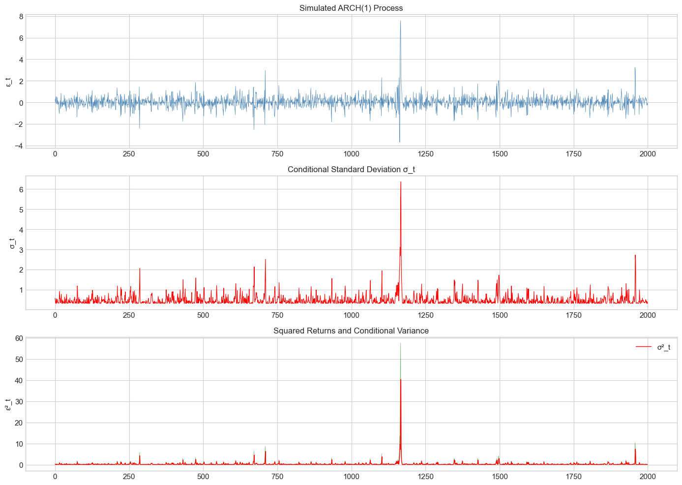
2. The GARCH Model
2.1 Motivation for GARCH
ARCH models require many lags to capture persistent volatility. Bollerslev (1986) introduced the Generalized ARCH (GARCH) model for parsimony.
2.2 GARCH(p,q) Specification
The GARCH(1,1) model is:
Interpretation:
: reaction coefficient (sensitivity to recent shocks)
: persistence coefficient (memory of past variance)
: overall persistence
2.3 GARCH as ARMA in Squared Returns
Define . Then GARCH(1,1) implies:
This is an ARMA(1,1) process in !
2.4 Stationarity and Persistence
Weak stationarity requires:
Unconditional variance:
Volatility half-life: Time for volatility shock to decay by half:
Source
def simulate_garch(n, omega, alphas, betas, dist='normal', df=5):
    """
    Simulate GARCH(p,q) process.

    Parameters
    ----------
    n : int
        Number of observations
    omega : float
        Constant term
    alphas : array-like
        ARCH coefficients
    betas : array-like
        GARCH coefficients
    dist : str
        Distribution of innovations
    df : int
        Degrees of freedom for t-distribution

    Returns
    -------
    eps, sigma2 : np.arrays
    """
    q = len(alphas)
    p = len(betas)
    max_lag = max(p, q)

    eps = np.zeros(n)
    sigma2 = np.zeros(n)

    if dist == 'normal':
        z = np.random.standard_normal(n)
    else:
        z = np.random.standard_t(df, n) / np.sqrt(df / (df - 2))

    # Unconditional variance
    uncond_var = omega / (1 - np.sum(alphas) - np.sum(betas))
    sigma2[:max_lag] = uncond_var
    eps[:max_lag] = np.sqrt(uncond_var) * z[:max_lag]

    for t in range(max_lag, n):
        arch_term = np.sum(alphas * eps[t-q:t][::-1]**2) if q > 0 else 0
        garch_term = np.sum(betas * sigma2[t-p:t][::-1]) if p > 0 else 0
        sigma2[t] = omega + arch_term + garch_term
        eps[t] = np.sqrt(sigma2[t]) * z[t]

    return eps, sigma2

# Compare ARCH(5) vs GARCH(1,1) with similar persistence
n = 2000

# ARCH(5) with persistence ≈ 0.85
alphas_arch5 = np.array([0.20, 0.20, 0.20, 0.15, 0.10])  # sum = 0.85
eps_arch5, sigma2_arch5 = simulate_arch(n, 0.1, alphas_arch5)

# GARCH(1,1) with persistence = 0.85
alpha_garch = 0.10
beta_garch = 0.85
eps_garch, sigma2_garch = simulate_garch(n, 0.1, [alpha_garch], [beta_garch])

fig, axes = plt.subplots(2, 2, figsize=(14, 8))

axes[0,0].plot(eps_arch5, color='steelblue', linewidth=0.5)
axes[0,0].set_title('ARCH(5) Returns', fontsize=12)

axes[0,1].plot(eps_garch, color='steelblue', linewidth=0.5)
axes[0,1].set_title('GARCH(1,1) Returns', fontsize=12)

axes[1,0].plot(np.sqrt(sigma2_arch5), color='red', linewidth=0.8)
axes[1,0].set_title('ARCH(5) Volatility', fontsize=12)

axes[1,1].plot(np.sqrt(sigma2_garch), color='red', linewidth=0.8)
axes[1,1].set_title('GARCH(1,1) Volatility', fontsize=12)

plt.tight_layout()
plt.suptitle('ARCH(5) vs GARCH(1,1): Same Persistence, Different Parameterization',
             y=1.02, fontsize=13, fontweight='bold')
plt.show()

print(f"ARCH(5): {len(alphas_arch5)+1} parameters")
print(f"GARCH(1,1): 3 parameters")
print(f"Both have persistence ≈ {np.sum(alphas_arch5):.2f}")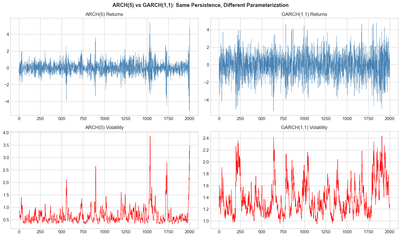
ARCH(5): 6 parameters
GARCH(1,1): 3 parameters
Both have persistence ≈ 0.85
3. Maximum Likelihood Estimation
3.1 The Likelihood Function
Assuming , the conditional density of is:
The log-likelihood function is:
3.2 Student-t Innovations
For heavier tails, use standardized Student-t distribution:
The log-likelihood becomes:
Source
def garch_log_likelihood(params, returns, p=1, q=1, dist='normal'):
    """
    Compute negative log-likelihood for GARCH(p,q) model.

    Parameters
    ----------
    params : array
        [omega, alpha_1,...,alpha_q, beta_1,...,beta_p, (df if t-dist)]
    returns : array
        Return series (demeaned)
    p : int
        GARCH order
    q : int
        ARCH order
    dist : str
        'normal' or 't'

    Returns
    -------
    float
        Negative log-likelihood
    """
    T = len(returns)
    omega = params[0]
    alphas = params[1:1+q]
    betas = params[1+q:1+q+p]

    if dist == 't':
        df = params[-1]
        if df <= 2:
            return 1e10

    # Check parameter constraints
    if omega <= 0 or np.any(alphas < 0) or np.any(betas < 0):
        return 1e10
    if np.sum(alphas) + np.sum(betas) >= 1:
        return 1e10

    # Initialize variance
    sigma2 = np.zeros(T)
    sigma2[0] = np.var(returns)  # Sample variance as initial

    # Compute conditional variances
    for t in range(1, T):
        sigma2[t] = omega
        for i in range(q):
            if t - i - 1 >= 0:
                sigma2[t] += alphas[i] * returns[t-i-1]**2
        for j in range(p):
            if t - j - 1 >= 0:
                sigma2[t] += betas[j] * sigma2[t-j-1]

    # Compute log-likelihood
    if dist == 'normal':
        ll = -0.5 * np.sum(np.log(2 * np.pi) + np.log(sigma2) + returns**2 / sigma2)
    else:  # t-distribution
        from scipy.special import gammaln
        ll = T * (gammaln((df+1)/2) - gammaln(df/2) - 0.5*np.log(np.pi*(df-2)))
        ll -= 0.5 * np.sum(np.log(sigma2))
        ll -= ((df+1)/2) * np.sum(np.log(1 + returns**2 / ((df-2)*sigma2)))

    return -ll  # Return negative for minimization


def fit_garch(returns, p=1, q=1, dist='normal'):
    """
    Fit GARCH(p,q) model by maximum likelihood.

    Returns
    -------
    dict with 'params', 'sigma2', 'loglik', 'aic', 'bic'
    """
    returns = np.asarray(returns)
    T = len(returns)

    # Initial parameter guesses
    var_returns = np.var(returns)
    omega_init = var_returns * 0.05
    alpha_init = [0.1] * q
    beta_init = [0.8 / p] * p

    if dist == 'normal':
        params_init = [omega_init] + alpha_init + beta_init
    else:
        params_init = [omega_init] + alpha_init + beta_init + [8.0]  # df

    # Optimize
    result = minimize(
        garch_log_likelihood,
        params_init,
        args=(returns, p, q, dist),
        method='Nelder-Mead',
        options={'maxiter': 10000}
    )

    # Refine with BFGS
    result = minimize(
        garch_log_likelihood,
        result.x,
        args=(returns, p, q, dist),
        method='BFGS',
        options={'maxiter': 5000}
    )

    params = result.x
    loglik = -result.fun

    # Compute fitted variances
    omega = params[0]
    alphas = params[1:1+q]
    betas = params[1+q:1+q+p]

    sigma2 = np.zeros(T)
    sigma2[0] = np.var(returns)

    for t in range(1, T):
        sigma2[t] = omega
        for i in range(q):
            if t - i - 1 >= 0:
                sigma2[t] += alphas[i] * returns[t-i-1]**2
        for j in range(p):
            if t - j - 1 >= 0:
                sigma2[t] += betas[j] * sigma2[t-j-1]

    # Information criteria
    k = len(params)
    aic = -2 * loglik + 2 * k
    bic = -2 * loglik + k * np.log(T)

    return {
        'params': params,
        'omega': omega,
        'alphas': alphas,
        'betas': betas,
        'sigma2': sigma2,
        'loglik': loglik,
        'aic': aic,
        'bic': bic,
        'persistence': np.sum(alphas) + np.sum(betas)
    }
Source
# Test on simulated data
true_omega = 0.05
true_alpha = 0.10
true_beta = 0.85

np.random.seed(42)
sim_returns, true_sigma2 = simulate_garch(2000, true_omega, [true_alpha], [true_beta])

# Fit GARCH(1,1)
result = fit_garch(sim_returns, p=1, q=1, dist='normal')

print("GARCH(1,1) Estimation Results (Simulated Data)")
print("="*50)
print(f"\nTrue parameters:")
print(f"  ω = {true_omega:.6f}")
print(f"  α = {true_alpha:.6f}")
print(f"  β = {true_beta:.6f}")
print(f"\nEstimated parameters:")
print(f"  ω = {result['omega']:.6f}")
print(f"  α = {result['alphas'][0]:.6f}")
print(f"  β = {result['betas'][0]:.6f}")
print(f"\nPersistence (α + β): {result['persistence']:.4f}")
print(f"Log-likelihood: {result['loglik']:.2f}")
GARCH(1,1) Estimation Results (Simulated Data)
==================================================
True parameters:
ω = 0.050000
α = 0.100000
β = 0.850000
Estimated parameters:
ω = 0.086825
α = 0.100369
β = 0.802914
Persistence (α + β): 0.9033
Log-likelihood: -2682.81
4. Empirical Application: S&P 500
Source
# Download S&P 500 data
spy = yf.download('SPY', start='2010-01-01', end='2024-12-31', progress=False)
if isinstance(spy.columns, pd.MultiIndex):
    spy.columns = spy.columns.get_level_values(0)

spy['returns'] = np.log(spy['Close'] / spy['Close'].shift(1))
returns = spy['returns'].dropna()

# Demean returns
returns_dm = returns - returns.mean()

print(f"Sample period: {returns.index[0].date()} to {returns.index[-1].date()}")
print(f"Number of observations: {len(returns)}")
print(f"Mean return: {returns.mean()*100:.4f}%")
print(f"Std deviation: {returns.std()*100:.4f}%")
print(f"Annualized volatility: {returns.std()*np.sqrt(252)*100:.2f}%")
YF.download() has changed argument auto_adjust default to True
Sample period: 2010-01-05 to 2024-12-30
Number of observations: 3772
Mean return: 0.0510%
Std deviation: 1.0774%
Annualized volatility: 17.10%
Source
# Use arch library for estimation with standard errors
from arch import arch_model

# Fit with arch library (scale returns to percentage for numerical stability)
model = arch_model(returns * 100, vol='Garch', p=1, q=1, dist='Normal')
fitted = model.fit(disp='off')

print("\nGARCH(1,1) Estimation (Normal innovations)")
print("="*50)
print(fitted.summary().tables[1])
GARCH(1,1) Estimation (Normal innovations)
==================================================
                                Mean Model
==========================================================================
                 coef    std err          t      P>|t|    95.0% Conf. Int.
--------------------------------------------------------------------------
mu             0.0864  1.216e-02      7.109  1.171e-12 [6.260e-02,  0.110]
==========================================================================
Source
# Compare with Student-t innovations
model_t = arch_model(returns * 100, vol='Garch', p=1, q=1, dist='t')
fitted_t = model_t.fit(disp='off')

print("\nGARCH(1,1) Estimation (Student-t innovations)")
print("="*50)
print(fitted_t.summary().tables[1])

print(f"\n\nModel Comparison:")
print(f"Normal:    AIC = {fitted.aic:.2f}, BIC = {fitted.bic:.2f}")
print(f"Student-t: AIC = {fitted_t.aic:.2f}, BIC = {fitted_t.bic:.2f}")
print(f"\nStudent-t degrees of freedom: {fitted_t.params['nu']:.2f}")
GARCH(1,1) Estimation (Student-t innovations)
==================================================
                                Mean Model
==========================================================================
                 coef    std err          t      P>|t|    95.0% Conf. Int.
--------------------------------------------------------------------------
mu             0.1023  1.057e-02      9.675  3.834e-22 [8.156e-02,  0.123]
==========================================================================


Model Comparison:
Normal:    AIC = 9650.08, BIC = 9675.02
Student-t: AIC = 9433.92, BIC = 9465.10

Student-t degrees of freedom: 5.51
Source
# Plot conditional volatility
fig, axes = plt.subplots(2, 1, figsize=(14, 8))

# Returns
axes[0].plot(returns.index, returns.values * 100, color='steelblue',
             linewidth=0.5, alpha=0.8)
axes[0].axhline(0, color='black', linewidth=0.5)
axes[0].set_ylabel('Return (%)')
axes[0].set_title('S&P 500 Daily Returns', fontsize=12)

# Conditional volatility
cond_vol = fitted.conditional_volatility
axes[1].plot(returns.index, cond_vol, color='red', linewidth=0.8)
axes[1].fill_between(returns.index, 0, cond_vol, color='red', alpha=0.2)
axes[1].set_ylabel('Conditional Volatility (%)')
axes[1].set_title('GARCH(1,1) Conditional Volatility', fontsize=12)
axes[1].set_xlabel('Date')

plt.tight_layout()
plt.show()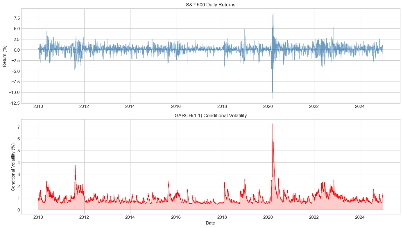
5. Model Diagnostics
5.1 Standardized Residuals
If the model is correctly specified, the standardized residuals:
should be i.i.d. with mean 0 and variance 1.
5.2 Diagnostic Tests
Ljung-Box test on : Test for remaining autocorrelation in returns
Ljung-Box test on : Test for remaining ARCH effects
Normality test: Jarque-Bera on
Source
from statsmodels.stats.diagnostic import acorr_ljungbox
from scipy.stats import jarque_bera
from statsmodels.graphics.tsaplots import plot_acf

def garch_diagnostics(fitted_model):
    """
    Perform diagnostic tests on GARCH residuals.
    """
    std_resid = fitted_model.std_resid

    print("GARCH Model Diagnostics")
    print("="*60)

    # Summary statistics of standardized residuals
    print("\n1. Standardized Residuals Summary:")
    print(f"   Mean: {std_resid.mean():.4f} (should be ≈ 0)")
    print(f"   Std:  {std_resid.std():.4f} (should be ≈ 1)")
    print(f"   Skew: {stats.skew(std_resid):.4f}")
    print(f"   Kurt: {stats.kurtosis(std_resid):.4f} (excess)")

    # Normality test
    jb_stat, jb_pval = jarque_bera(std_resid)
    print(f"\n2. Jarque-Bera Normality Test:")
    print(f"   Statistic: {jb_stat:.2f}")
    print(f"   p-value:   {jb_pval:.6f}")
    print(f"   Result:    {'Reject H0 (non-normal)' if jb_pval < 0.05 else 'Fail to reject H0'}")

    # Ljung-Box on standardized residuals
    lb_resid = acorr_ljungbox(std_resid, lags=[10, 20], return_df=True)
    print(f"\n3. Ljung-Box Test on Standardized Residuals:")
    print(f"   Lag 10: Q = {lb_resid['lb_stat'].iloc[0]:.2f}, p = {lb_resid['lb_pvalue'].iloc[0]:.4f}")
    print(f"   Lag 20: Q = {lb_resid['lb_stat'].iloc[1]:.2f}, p = {lb_resid['lb_pvalue'].iloc[1]:.4f}")

    # Ljung-Box on squared standardized residuals (ARCH effects)
    lb_sq = acorr_ljungbox(std_resid**2, lags=[10, 20], return_df=True)
    print(f"\n4. Ljung-Box Test on Squared Standardized Residuals:")
    print(f"   Lag 10: Q = {lb_sq['lb_stat'].iloc[0]:.2f}, p = {lb_sq['lb_pvalue'].iloc[0]:.4f}")
    print(f"   Lag 20: Q = {lb_sq['lb_stat'].iloc[1]:.2f}, p = {lb_sq['lb_pvalue'].iloc[1]:.4f}")

    return std_resid

std_resid = garch_diagnostics(fitted)
GARCH Model Diagnostics
============================================================
1. Standardized Residuals Summary:
Mean: -0.0509 (should be ≈ 0)
Std: 0.9986 (should be ≈ 1)
Skew: -0.6267
Kurt: 1.8564 (excess)
2. Jarque-Bera Normality Test:
Statistic: 788.54
p-value: 0.000000
Result: Reject H0 (non-normal)
3. Ljung-Box Test on Standardized Residuals:
Lag 10: Q = 11.65, p = 0.3088
Lag 20: Q = 25.22, p = 0.1930
4. Ljung-Box Test on Squared Standardized Residuals:
Lag 10: Q = 7.41, p = 0.6860
Lag 20: Q = 10.70, p = 0.9537
Source
# Visual diagnostics
fig, axes = plt.subplots(2, 2, figsize=(14, 10))

# Time series of standardized residuals
axes[0,0].plot(returns.index, std_resid, color='steelblue', linewidth=0.5)
axes[0,0].axhline(0, color='black', linewidth=0.5)
axes[0,0].axhline(2, color='red', linestyle='--', alpha=0.5)
axes[0,0].axhline(-2, color='red', linestyle='--', alpha=0.5)
axes[0,0].set_title('Standardized Residuals', fontsize=12)
axes[0,0].set_ylabel('z_t')

# Histogram vs Normal
axes[0,1].hist(std_resid, bins=100, density=True, alpha=0.7,
               color='steelblue', edgecolor='white')
x = np.linspace(-5, 5, 100)
axes[0,1].plot(x, norm.pdf(x), 'r-', lw=2, label='Normal')
axes[0,1].set_title('Distribution of Standardized Residuals', fontsize=12)
axes[0,1].legend()

# ACF of standardized residuals
plot_acf(std_resid, lags=30, ax=axes[1,0], alpha=0.05)
axes[1,0].set_title('ACF of Standardized Residuals', fontsize=12)

# ACF of squared standardized residuals
plot_acf(std_resid**2, lags=30, ax=axes[1,1], alpha=0.05)
axes[1,1].set_title('ACF of Squared Standardized Residuals', fontsize=12)

plt.tight_layout()
plt.show()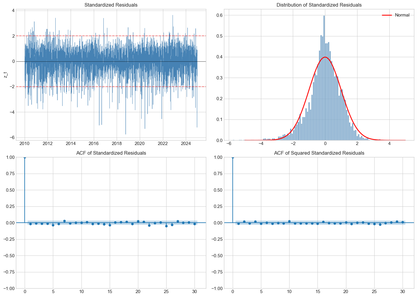
6. Model Selection
6.1 Information Criteria
Akaike Information Criterion (AIC):
Bayesian Information Criterion (BIC):
where is the number of parameters and is the sample size.
BIC penalizes complexity more heavily and tends to select more parsimonious models.
Source
# Model selection: Compare different GARCH specifications
specifications = [
    (1, 1, 'Normal'),
    (1, 1, 't'),
    (1, 2, 'Normal'),
    (1, 2, 't'),
    (2, 1, 'Normal'),
    (2, 1, 't'),
    (2, 2, 'Normal'),
    (2, 2, 't'),
]

results = []
for p, q, dist in specifications:
    model = arch_model(returns * 100, vol='Garch', p=p, q=q, dist=dist)
    fit = model.fit(disp='off')
    results.append({
        'Model': f'GARCH({p},{q})',
        'Distribution': dist,
        'Log-Lik': fit.loglikelihood,
        'AIC': fit.aic,
        'BIC': fit.bic,
        'Params': fit.num_params
    })

results_df = pd.DataFrame(results)
results_df = results_df.sort_values('BIC')

print("Model Selection Results")
print("="*70)
print(results_df.to_string(index=False))
print(f"\nBest model by BIC: {results_df.iloc[0]['Model']} with {results_df.iloc[0]['Distribution']} innovations")
Model Selection Results
======================================================================
Model Distribution Log-Lik AIC BIC Params
GARCH(1,1) t -4711.959934 9433.919868 9465.096671 5
GARCH(2,1) t -4708.599087 9429.198175 9466.610339 6
GARCH(1,2) t -4711.959934 9435.919868 9473.332032 6
GARCH(2,2) t -4708.324808 9430.649616 9474.297140 7
GARCH(1,1) Normal -4821.041592 9650.083185 9675.024628 4
GARCH(2,1) Normal -4819.078583 9648.157167 9679.333970 5
GARCH(1,2) Normal -4821.041593 9652.083185 9683.259988 5
GARCH(2,2) Normal -4818.129509 9648.259018 9685.671182 6
Best model by BIC: GARCH(1,1) with t innovations
7. Volatility Forecasting
7.1 Multi-Step Forecasts
For GARCH(1,1), the h-step ahead forecast is:
where is the unconditional variance.
As , .
7.2 Forecast Evaluation
Since volatility is latent, we need proxies:
Squared returns: (noisy but unbiased)
Realized variance (high-frequency data)
Implied volatility (from options)
Source
# Generate volatility forecasts
forecast_horizon = 22  # 1 month ahead

# Fit model on data up to a point and forecast
train_end = '2023-12-31'
returns_train = returns[returns.index <= train_end]
returns_test = returns[returns.index > train_end]

model = arch_model(returns_train * 100, vol='Garch', p=1, q=1, dist='t')
fitted = model.fit(disp='off')

# Multi-step forecast
forecasts = fitted.forecast(horizon=forecast_horizon, reindex=False)

print("Volatility Forecasts (% per day)")
print("="*40)
print(f"1-day ahead: {np.sqrt(forecasts.variance.iloc[-1, 0]):.4f}%")
print(f"5-day ahead: {np.sqrt(forecasts.variance.iloc[-1, 4]):.4f}%")
print(f"22-day ahead: {np.sqrt(forecasts.variance.iloc[-1, -1]):.4f}%")

# Unconditional volatility
omega = fitted.params['omega']
alpha = fitted.params['alpha[1]']
beta = fitted.params['beta[1]']
uncond_vol = np.sqrt(omega / (1 - alpha - beta))
print(f"\nUnconditional volatility: {uncond_vol:.4f}%")
Volatility Forecasts (% per day)
========================================
1-day ahead: 0.6337%
5-day ahead: 0.6960%
22-day ahead: 0.9023%
Unconditional volatility: 1.9216%
Source
# Rolling forecast evaluation
def rolling_forecast_evaluation(returns, window=1000, horizon=1):
    """
    Perform rolling 1-step ahead forecasts and compare to realized volatility.
    """
    forecasted_vol = []
    realized_vol = []
    dates = []

    returns_array = returns * 100  # Convert to percentage

    for t in range(window, len(returns_array) - horizon):
        # Fit on rolling window
        train = returns_array.iloc[t-window:t]

        try:
            model = arch_model(train, vol='Garch', p=1, q=1, dist='Normal')
            fit = model.fit(disp='off', show_warning=False)

            # 1-step forecast
            fcast = fit.forecast(horizon=horizon, reindex=False)
            forecasted_vol.append(np.sqrt(fcast.variance.iloc[-1, -1]))

            # Realized volatility proxy: absolute return
            realized_vol.append(np.abs(returns_array.iloc[t + horizon - 1]))
            dates.append(returns_array.index[t + horizon - 1])
        except:
            continue

    return pd.DataFrame({
        'forecasted': forecasted_vol,
        'realized': realized_vol
    }, index=dates)

# Run rolling evaluation (subset for speed)
returns_subset = returns['2020-01-01':'2024-12-31']
eval_df = rolling_forecast_evaluation(returns_subset, window=500, horizon=1)

# Compute forecast evaluation metrics
mse = np.mean((eval_df['forecasted'] - eval_df['realized'])**2)
mae = np.mean(np.abs(eval_df['forecasted'] - eval_df['realized']))
corr = eval_df['forecasted'].corr(eval_df['realized'])

print("Forecast Evaluation (1-day ahead)")
print("="*40)
print(f"MSE: {mse:.4f}")
print(f"MAE: {mae:.4f}")
print(f"Correlation: {corr:.4f}")
Forecast Evaluation (1-day ahead)
========================================
MSE: 0.5660
MAE: 0.6038
Correlation: 0.3263
Source
# Plot forecast vs realized
fig, axes = plt.subplots(2, 1, figsize=(14, 8))

# Time series comparison
axes[0].plot(eval_df.index, eval_df['forecasted'], color='red',
             linewidth=0.8, label='Forecasted σ', alpha=0.8)
axes[0].plot(eval_df.index, eval_df['realized'], color='steelblue',
             linewidth=0.5, label='|Return|', alpha=0.5)
axes[0].set_title('GARCH(1,1) Volatility Forecast vs Realized', fontsize=12)
axes[0].set_ylabel('Volatility (%)')
axes[0].legend()

# Scatter plot
axes[1].scatter(eval_df['forecasted'], eval_df['realized'],
                alpha=0.2, s=10, color='steelblue')
axes[1].plot([0, eval_df['forecasted'].max()], [0, eval_df['forecasted'].max()],
             'r--', linewidth=1, label='45° line')
axes[1].set_xlabel('Forecasted Volatility (%)')
axes[1].set_ylabel('Realized |Return| (%)')
axes[1].set_title(f'Forecast vs Realized (Correlation: {corr:.3f})', fontsize=12)
axes[1].legend()

plt.tight_layout()
plt.show()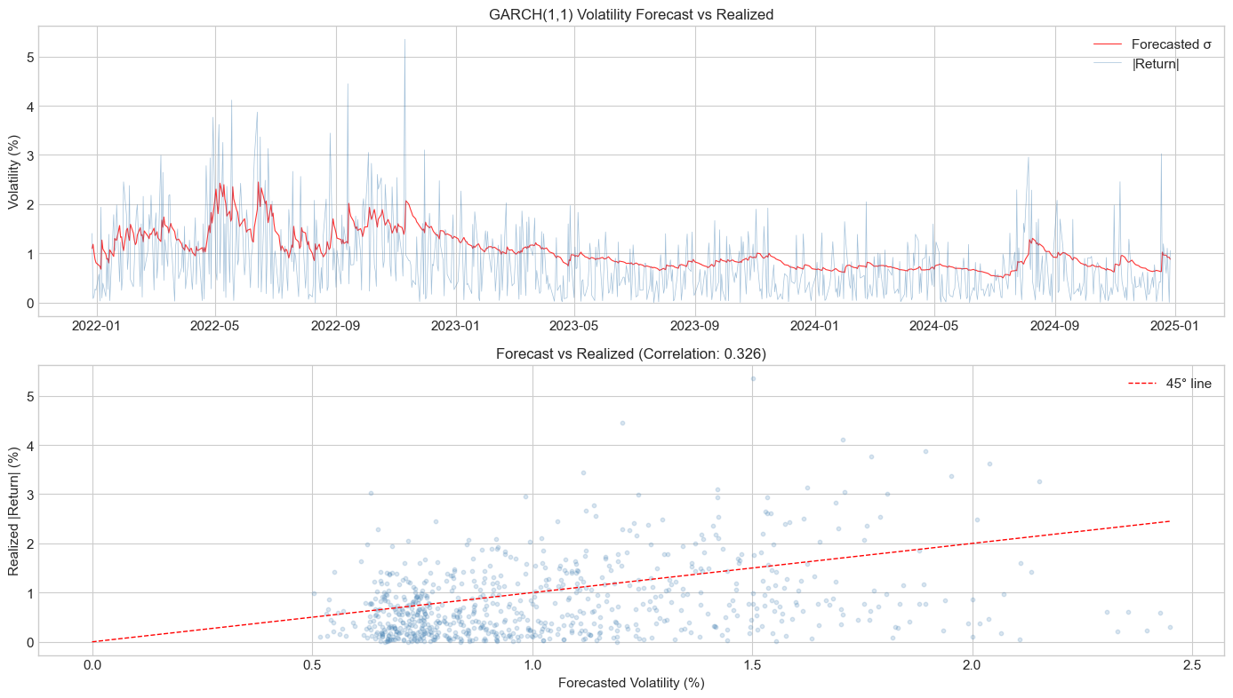
8. Integrated GARCH (IGARCH)
When , we have the Integrated GARCH model. This implies:
Shocks to volatility persist forever
Unconditional variance is infinite
Volatility forecasts don’t revert to a long-run mean
The EWMA model is a special case: IGARCH(1,1) with no constant:
where and .
Source
# Compare GARCH vs IGARCH forecasts
# Standard GARCH(1,1)
model_garch = arch_model(returns * 100, vol='Garch', p=1, q=1)
fit_garch = model_garch.fit(disp='off')

# EWMA (RiskMetrics) - IGARCH with lambda=0.94
model_ewma = arch_model(returns * 100, vol='EWMA')#, lam=0.94)
fit_ewma = model_ewma.fit(disp='off')

# Generate long-horizon forecasts
horizon = 100
fcast_garch = fit_garch.forecast(horizon=horizon, reindex=False)
fcast_ewma = fit_ewma.forecast(horizon=horizon, reindex=False)

# Plot forecast paths
fig, ax = plt.subplots(figsize=(12, 6))

days = np.arange(1, horizon + 1)
ax.plot(days, np.sqrt(fcast_garch.variance.iloc[-1].values),
        'b-', linewidth=2, label='GARCH(1,1)')
ax.plot(days, np.sqrt(fcast_ewma.variance.iloc[-1].values),
        'r--', linewidth=2, label='EWMA (λ=0.94)')

# Unconditional volatility
omega = fit_garch.params['omega']
alpha = fit_garch.params['alpha[1]']
beta = fit_garch.params['beta[1]']
uncond_vol = np.sqrt(omega / (1 - alpha - beta))
ax.axhline(uncond_vol, color='blue', linestyle=':', alpha=0.5,
           label=f'GARCH unconditional vol: {uncond_vol:.2f}%')

ax.set_xlabel('Forecast Horizon (days)')
ax.set_ylabel('Forecasted Volatility (%)')
ax.set_title('GARCH vs IGARCH (EWMA): Forecast Mean Reversion', fontsize=13)
ax.legend()

plt.tight_layout()
plt.show()

print(f"\nGARCH(1,1) persistence: {alpha + beta:.4f}")
print(f"EWMA persistence: 1.0000 (by construction)")
---------------------------------------------------------------------------
ValueError Traceback (most recent call last)
Cell In[41], line 7
4 fit_garch = model_garch.fit(disp='off')
6 # EWMA (RiskMetrics) - IGARCH with lambda=0.94
----> 7 model_ewma = arch_model(returns * 100, vol='EWMA')#, lam=0.94)
8 fit_ewma = model_ewma.fit(disp='off')
10 # Generate long-horizon forecasts
File ~\AppData\Local\anaconda3\Lib\site-packages\arch\univariate\mean.py:2019, in arch_model(y, x, mean, lags, vol, p, o, q, power, dist, hold_back, rescale)
2017 raise ValueError("Unknown model type in mean")
2018 if vol_model not in known_vol:
-> 2019 raise ValueError("Unknown model type in vol")
2020 if dist_name not in known_dist:
2021 raise ValueError("Unknown model type in dist")
ValueError: Unknown model type in vol9. Summary
Key Takeaways
ARCH models capture volatility clustering by making variance depend on past squared shocks
GARCH extends ARCH with lagged variance terms, providing a parsimonious representation
Estimation is done by maximum likelihood; Student-t innovations typically improve fit
Diagnostics check that standardized residuals are i.i.d.
GARCH(1,1) is often sufficient for daily financial data
Persistence () determines how quickly volatility reverts to its mean
Preview of Session 3
GARCH(1,1) has a symmetric news impact: positive and negative shocks of the same magnitude have the same effect on volatility. But we know the leverage effect exists!
Session 3 covers asymmetric GARCH models: EGARCH, GJR-GARCH, TGARCH.
Exercises
Exercise 1: Bitcoin GARCH
Fit GARCH(1,1) to Bitcoin daily returns. How does the persistence compare to S&P 500? What does this imply about volatility half-life?
Exercise 2: Distribution Choice
Compare Normal, Student-t, and Skewed Student-t distributions for S&P 500. Which provides the best fit according to BIC?
Exercise 3: Higher-Order GARCH
Estimate GARCH(2,2) for S&P 500. Is the improvement in log-likelihood worth the additional parameters?
Exercise 4: Forecast Evaluation
Implement the Mincer-Zarnowitz regression:
Test H0: (unbiased forecasts).
Exercise 5: IGARCH
Fit IGARCH(1,1) to S&P 500 and compare forecasts with GARCH(1,1) at horizons of 1, 5, 22, and 66 days.
References
Engle, R. F. (1982). Autoregressive conditional heteroscedasticity with estimates of the variance of United Kingdom inflation. Econometrica, 50(4), 987-1007.
Bollerslev, T. (1986). Generalized autoregressive conditional heteroskedasticity. Journal of Econometrics, 31(3), 307-327.
Bollerslev, T., Chou, R. Y., & Kroner, K. F. (1992). ARCH modeling in finance: A review of the theory and empirical evidence. Journal of Econometrics, 52(1-2), 5-59.
Francq, C., & Zakoian, J. M. (2019). GARCH Models: Structure, Statistical Inference and Financial Applications. John Wiley & Sons.