Lecture 5: Fixed-Income Securities II — Duration, Convexity, Credit Risk, and Securitization

MIT 15.401 — Finance Theory I (Prof. Andrew Lo)¶

Video: MIT OCW — Part III & IV of Fixed-Income Securities

Readings: Brealey, Myers, and Allen — Chapters 23–25; Sundaresan, Fixed Income Markets and Their Derivatives

This notebook completes the Fixed-Income Securities block (Sessions 4–7 in Lo’s numbering). We move from bond pricing to risk measurement, asking: once you own a bond, how sensitive is your position to changes in interest rates? The answers — duration and convexity — are the foundational tools of fixed-income risk management.

We then shift from riskless government debt to corporate bonds, where default risk introduces an entirely new dimension. The session culminates with Lo’s remarkable real-time case study of the sub-prime crisis and securitization, taught as Lehman Brothers was collapsing. His simple two-bond CDO example demonstrates how correlation assumptions can destroy the supposed safety of senior tranches — the mechanism at the heart of the 2008 financial crisis.

Table of Contents¶

# ============================================================
# Setup
# ============================================================
import numpy as np
import pandas as pd
import matplotlib.pyplot as plt
import matplotlib.ticker as mticker
from scipy.optimize import brentq
from IPython.display import display, Markdown

plt.rcParams.update({
    'figure.figsize': (10, 5),
    'axes.spines.top': False,
    'axes.spines.right': False,
    'axes.grid': True,
    'grid.alpha': 0.3,
    'font.size': 12,
    'lines.linewidth': 2,
})

# Bond toolkit from Session 4
def bond_price_from_ytm(face, coupon_rate, maturity, ytm, freq=1):
    C = face * coupon_rate / freq
    n = maturity * freq
    y = ytm / freq
    price = sum(C / (1 + y)**t for t in range(1, n + 1))
    price += face / (1 + y)**n
    return price

def compute_ytm(price, face, coupon_rate, maturity, freq=1):
    def f(y):
        return bond_price_from_ytm(face, coupon_rate, maturity, y, freq) - price
    return brentq(f, -0.05, 2.0)

print("Libraries and bond toolkit loaded.")

Libraries and bond toolkit loaded.

1. Macaulay Duration¶

Motivation¶

We showed in Session 4 that bond prices move inversely with yields. But how much does a bond’s price change for a given yield movement? This is the central question of interest rate risk management.

Frederick Macaulay (1938) proposed an elegant answer: duration — a single number that captures a bond’s price sensitivity to yield changes.

Definition¶

Macaulay duration $D$ is the weighted average time to receipt of cash flows, where the weights are the present values of each cash flow as a fraction of the bond price:

\boxed{D = \sum_{k=1}^{T} k \cdot \omega_k}

(1)

where

\omega_k = \frac{PV(CF_k)}{P} = \frac{CF_k / (1+y)^k}{P}, \qquad \sum_{k=1}^{T} \omega_k = 1

(2)

Duration is measured in years (or half-years for semi-annual bonds). It tells you the bond’s “effective maturity” — the average time you wait to receive your money, weighted by economic importance.

Key Properties of Macaulay Duration¶

Zero-coupon bond: $D = T$ (all weight on the single payment at maturity)
Coupon bond: $D < T$ (coupons pull the weighted average inward)
Duration decreases with coupon rate (more early cash flows)
Duration decreases with YTM (higher discounting reduces weight of distant flows)
Duration usually increases with maturity (for bonds at or above par, always; for deep discount bonds, can decrease — rare in practice)
Perpetuity: $D = (1+y)/y$

# ============================================================
# Macaulay Duration Calculation
# ============================================================

def macaulay_duration(face, coupon_rate, maturity, ytm, freq=1):
    """Compute Macaulay duration.
    
    For semi-annual bonds (freq=2), returns duration in YEARS
    (i.e., divides by freq at the end).
    """
    C = face * coupon_rate / freq
    n = maturity * freq
    y = ytm / freq
    
    price = bond_price_from_ytm(face, coupon_rate, maturity, ytm, freq)
    
    weighted_sum = 0
    for k in range(1, n + 1):
        cf = C if k < n else C + face
        pv_cf = cf / (1 + y)**k
        weighted_sum += k * pv_cf
    
    return weighted_sum / (price * freq)  # Convert to annual


# Lo's example from slide 37: 4-year T-note, 7% coupon, 6% yield, semi-annual
face = 100
coupon_rate = 0.07
maturity = 4
ytm = 0.06
freq = 2

C = face * coupon_rate / freq  # 3.5 semi-annual coupon
n = maturity * freq             # 8 periods
y = ytm / freq                  # 3% per period

price = bond_price_from_ytm(face, coupon_rate, maturity, ytm, freq)
D = macaulay_duration(face, coupon_rate, maturity, ytm, freq)

print("=" * 75)
print("MACAULAY DURATION — Lo's T-Note Example")
print(f"4-Year T-Note, {coupon_rate:.0%} coupon (semi-annual), YTM = {ytm:.0%}")
print("=" * 75)
print(f"{'Period k':>10s} {'CF':>8s} {'PV(CF)':>12s} {'Weight ωk':>12s} {'k × ωk':>12s}")
print("-" * 55)

total_w = 0
total_kw = 0
for k in range(1, n + 1):
    cf = C if k < n else C + face
    pv_cf = cf / (1 + y)**k
    w = pv_cf / price
    kw = k * w
    total_w += w
    total_kw += kw
    print(f"{k:>10d} {cf:>8.2f} {pv_cf:>12.4f} {w:>12.6f} {kw:>12.6f}")

print("-" * 55)
print(f"{'SUM':>10s} {'':>8s} {price:>12.4f} {total_w:>12.6f} {total_kw:>12.6f}")
print(f"\nMacaulay Duration (half-year units): D = {total_kw:.2f} half-years")
print(f"Macaulay Duration (annual):          D = {total_kw / freq:.2f} years")
print(f"Bond Price: ${price:.2f} (per $100 face)")

===========================================================================
MACAULAY DURATION — Lo's T-Note Example
4-Year T-Note, 7% coupon (semi-annual), YTM = 6%
===========================================================================
  Period k       CF       PV(CF)    Weight ωk       k × ωk
-------------------------------------------------------
         1     3.50       3.3981     0.032828     0.032828
         2     3.50       3.2991     0.031872     0.063744
         3     3.50       3.2030     0.030944     0.092832
         4     3.50       3.1097     0.030043     0.120170
         5     3.50       3.0191     0.029168     0.145838
         6     3.50       2.9312     0.028318     0.169908
         7     3.50       2.8458     0.027493     0.192453
         8   103.50      81.7039     0.789334     6.314673
-------------------------------------------------------
       SUM              103.5098     1.000000     7.132447

Macaulay Duration (half-year units): D = 7.13 half-years
Macaulay Duration (annual):          D = 3.57 years
Bond Price: $103.51 (per $100 face)

# ============================================================
# Duration Weights — Visualization
# ============================================================
weights = []
periods = list(range(1, n + 1))
for k in periods:
    cf = C if k < n else C + face
    pv_cf = cf / (1 + y)**k
    weights.append(pv_cf / price)

fig, ax = plt.subplots(figsize=(12, 6))
colors = ['#3498db'] * (n - 1) + ['#e74c3c']
ax.bar(periods, weights, color=colors, alpha=0.8, edgecolor='white', width=0.7)

# Duration line
D_halfyears = sum(k * w for k, w in zip(periods, weights))
ax.axvline(x=D_halfyears, color='#e67e22', linewidth=3, linestyle='--',
           label=f'Duration = {D_halfyears:.2f} half-years ({D_halfyears/2:.2f} years)')

# Fulcrum analogy
ax.annotate('Duration = "balance point"\nof the PV-weighted\ncash flow timeline',
            xy=(D_halfyears, max(weights) * 0.4),
            xytext=(D_halfyears + 1.5, max(weights) * 0.6),
            fontsize=10, color='#e67e22', style='italic',
            arrowprops=dict(arrowstyle='->', color='#e67e22', lw=2),
            bbox=dict(boxstyle='round,pad=0.4', facecolor='#fdf6e3', alpha=0.9))

ax.set_xlabel('Period (half-years)', fontsize=12)
ax.set_ylabel('Weight ωk', fontsize=12)
ax.set_title(f'Duration Weights: 4-Year, {coupon_rate:.0%} Coupon T-Note (YTM = {ytm:.0%})',
             fontsize=14, fontweight='bold')
ax.legend(fontsize=12)
ax.set_xticks(periods)

plt.tight_layout()
plt.show()

print("The last bar (period 8) is much larger because it includes the principal repayment.")
print(f"Weight on final period: {weights[-1]:.1%} of total PV")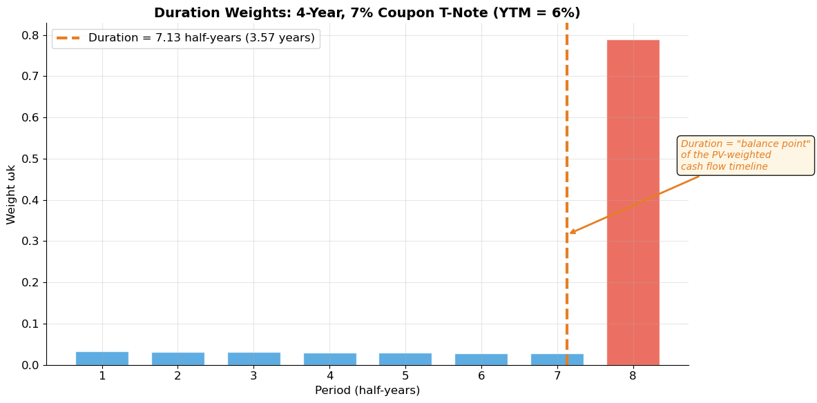

The last bar (period 8) is much larger because it includes the principal repayment.
Weight on final period: 78.9% of total PV

2. Modified Duration and Dollar Duration¶

From Duration to Price Sensitivity¶

The mathematical connection between Macaulay duration and price sensitivity comes from calculus. Taking the derivative of the bond price with respect to yield:

\frac{1}{P} \frac{\partial P}{\partial y} = -\frac{D}{1 + y/q}

(3)

where $q$ is the compounding frequency per year.

Modified Duration¶

Modified duration $D^*$ adjusts Macaulay duration for the compounding frequency:

\boxed{D^* = \frac{D}{1 + y/q}}

(4)

Modified duration gives us the percentage price change for a small yield change:

\frac{\Delta P}{P} \approx -D^* \times \Delta y

(5)

Dollar Duration¶

Sometimes we want the dollar (not percentage) price change:

\boxed{\Delta P \approx -D^* \times P \times \Delta y}

(6)

The quantity $D^* \times P$ is called the dollar duration or DV01 (dollar value of one basis point, when $\Delta y = 0.0001$ ).

# ============================================================
# Modified Duration and Price Sensitivity
# ============================================================

def modified_duration(face, coupon_rate, maturity, ytm, freq=1):
    D = macaulay_duration(face, coupon_rate, maturity, ytm, freq)
    return D / (1 + ytm / freq)

def dollar_duration(face, coupon_rate, maturity, ytm, freq=1):
    price = bond_price_from_ytm(face, coupon_rate, maturity, ytm, freq)
    Dmod = modified_duration(face, coupon_rate, maturity, ytm, freq)
    return Dmod * price

# Lo's example continued
D_mac = macaulay_duration(100, 0.07, 4, 0.06, 2)
D_mod = modified_duration(100, 0.07, 4, 0.06, 2)
price_base = bond_price_from_ytm(100, 0.07, 4, 0.06, 2)
DD = dollar_duration(100, 0.07, 4, 0.06, 2)
DV01 = DD * 0.0001

print("=" * 60)
print("MODIFIED DURATION — Lo's T-Note Example")
print("=" * 60)
print(f"Macaulay Duration:  D  = {D_mac:.4f} years")
print(f"Modified Duration:  D* = D/(1+y/2) = {D_mac:.4f}/{1+0.03:.2f} = {D_mod:.4f}")
print(f"Bond Price:         P  = ${price_base:.4f}")
print(f"Dollar Duration:    D* × P = {D_mod:.4f} × {price_base:.4f} = {DD:.4f}")
print(f"DV01 (per $100):    {DV01:.4f}")

# Price change prediction
dy = 0.001  # 10 basis points
predicted_change = -D_mod * dy * 100  # in percentage
actual_new_price = bond_price_from_ytm(100, 0.07, 4, 0.06 + dy, 2)
actual_change = (actual_new_price - price_base) / price_base * 100

print(f"\nIf yield rises by {dy*10000:.0f} bps ({dy:.2%}):")
print(f"  Duration approximation: ΔP/P ≈ -{D_mod:.4f} × {dy} = {predicted_change:+.4f}%")
print(f"  Actual price change:    ΔP/P = {actual_change:+.4f}%")
print(f"  Approximation error:    {abs(predicted_change - actual_change):.4f} percentage points")

# Larger move
dy2 = 0.02  # 200 bps
pred2 = -D_mod * dy2 * 100
actual2 = (bond_price_from_ytm(100, 0.07, 4, 0.06 + dy2, 2) - price_base) / price_base * 100
print(f"\nIf yield rises by {dy2*10000:.0f} bps ({dy2:.1%}):")
print(f"  Duration approximation: ΔP/P ≈ {pred2:+.4f}%")
print(f"  Actual price change:    ΔP/P = {actual2:+.4f}%")
print(f"  Approximation error:    {abs(pred2 - actual2):.4f} pp  ← error grows for large moves!")

============================================================
MODIFIED DURATION — Lo's T-Note Example
============================================================
Macaulay Duration:  D  = 3.5662 years
Modified Duration:  D* = D/(1+y/2) = 3.5662/1.03 = 3.4624
Bond Price:         P  = $103.5098
Dollar Duration:    D* × P = 3.4624 × 103.5098 = 358.3876
DV01 (per $100):    0.0358

If yield rises by 10 bps (0.10%):
  Duration approximation: ΔP/P ≈ -3.4624 × 0.001 = -0.3462%
  Actual price change:    ΔP/P = -0.3455%
  Approximation error:    0.0007 percentage points

If yield rises by 200 bps (2.0%):
  Duration approximation: ΔP/P ≈ -6.9247%
  Actual price change:    ΔP/P = -6.6431%
  Approximation error:    0.2816 pp  ← error grows for large moves!

# ============================================================
# Duration Across Bond Types — Comparative Analysis
# ============================================================
print("=" * 75)
print("DURATION COMPARISON ACROSS BOND TYPES")
print("=" * 75)
print(f"{'Bond':>30s} {'Price':>8s} {'Mac D':>8s} {'Mod D':>8s} {'DV01':>8s}")
print("-" * 75)

bonds = [
    ('Zero-coupon, 5yr',        1000, 0.00, 5,  0.05, 1),
    ('Zero-coupon, 10yr',       1000, 0.00, 10, 0.05, 1),
    ('Zero-coupon, 30yr',       1000, 0.00, 30, 0.05, 1),
    ('3% coupon, 10yr',         1000, 0.03, 10, 0.05, 1),
    ('5% coupon, 10yr (par)',   1000, 0.05, 10, 0.05, 1),
    ('8% coupon, 10yr',         1000, 0.08, 10, 0.05, 1),
    ('5% coupon, 2yr',          1000, 0.05, 2,  0.05, 1),
    ('5% coupon, 30yr',         1000, 0.05, 30, 0.05, 1),
    ('7% semi-annual, 4yr',     100,  0.07, 4,  0.06, 2),
]

results = []
for name, F, c, T, y, freq in bonds:
    P = bond_price_from_ytm(F, c, T, y, freq)
    Dm = macaulay_duration(F, c, T, y, freq)
    Dmod = modified_duration(F, c, T, y, freq)
    dv01 = Dmod * P * 0.0001
    results.append((name, P, Dm, Dmod, dv01, T))
    # Normalize price to per-100
    P_100 = P / F * 100 if F != 100 else P
    dv01_100 = dv01 / F * 100 if F != 100 else dv01
    print(f"{name:>30s} {P_100:>8.2f} {Dm:>8.2f} {Dmod:>8.2f} {dv01_100:>8.4f}")

print("\nKey patterns:")
print("• Zero-coupon: D = T always (no coupons to pull weighted average inward)")
print("• Higher coupon → lower duration (more early cash flows)")
print("• Longer maturity → higher duration (usually)")
print("• Higher yield → lower duration (distant cash flows discounted more heavily)")

===========================================================================
DURATION COMPARISON ACROSS BOND TYPES
===========================================================================
                          Bond    Price    Mac D    Mod D     DV01
---------------------------------------------------------------------------
              Zero-coupon, 5yr    78.35     5.00     4.76   0.0373
             Zero-coupon, 10yr    61.39    10.00     9.52   0.0585
             Zero-coupon, 30yr    23.14    30.00    28.57   0.0661
               3% coupon, 10yr    84.56     8.66     8.25   0.0697
         5% coupon, 10yr (par)   100.00     8.11     7.72   0.0772
               8% coupon, 10yr   123.17     7.54     7.18   0.0885
                5% coupon, 2yr   100.00     1.95     1.86   0.0186
               5% coupon, 30yr   100.00    16.14    15.37   0.1537
           7% semi-annual, 4yr   103.51     3.57     3.46   0.0358

Key patterns:
• Zero-coupon: D = T always (no coupons to pull weighted average inward)
• Higher coupon → lower duration (more early cash flows)
• Longer maturity → higher duration (usually)
• Higher yield → lower duration (distant cash flows discounted more heavily)

3. Convexity¶

Why Duration Isn’t Enough¶

Duration gives us a linear approximation to the price-yield relationship. But we know from Session 4 that this relationship is curved (convex). For large yield changes, the linear approximation becomes inaccurate.

Definition¶

Convexity $V$ measures the curvature — it is the second derivative of the price with respect to yield, normalized by price:

\boxed{V = \frac{1}{P} \frac{\partial^2 P}{\partial y^2} = \frac{1}{(1+y/q)^2} \sum_{k=1}^{T} \frac{k(k+1) \cdot CF_k}{q^2 \cdot P \cdot (1 + y/q)^k}}

(7)

Key Properties¶

Convexity is always positive for standard bonds (no embedded options)
Higher convexity is desirable: for the same duration, a more convex bond gains more when yields fall and loses less when yields rise — a “free lunch” in interest rate risk
Longer maturity → higher convexity
Lower coupon → higher convexity (same pattern as duration)

# ============================================================
# Convexity Calculation
# ============================================================

def bond_convexity(face, coupon_rate, maturity, ytm, freq=1):
    """Compute convexity (annualized)."""
    C = face * coupon_rate / freq
    n = maturity * freq
    y = ytm / freq
    price = bond_price_from_ytm(face, coupon_rate, maturity, ytm, freq)
    
    conv_sum = 0
    for k in range(1, n + 1):
        cf = C if k < n else C + face
        conv_sum += k * (k + 1) * cf / (1 + y)**k
    
    return conv_sum / (price * freq**2 * (1 + y)**2)


# Lo's example
V = bond_convexity(100, 0.07, 4, 0.06, 2)
D_mod_lo = modified_duration(100, 0.07, 4, 0.06, 2)
P_lo = bond_price_from_ytm(100, 0.07, 4, 0.06, 2)

print("=" * 60)
print("CONVEXITY — Lo's T-Note Example")
print("=" * 60)
print(f"Modified Duration: D* = {D_mod_lo:.6f}")
print(f"Convexity:         V  = {V:.6f}")
print(f"Bond Price:        P  = ${P_lo:.4f}")

============================================================
CONVEXITY — Lo's T-Note Example
============================================================
Modified Duration: D* = 3.462353
Convexity:         V  = 14.531325
Bond Price:        P  = $103.5098

4. The Duration-Convexity Approximation¶

The Second-Order Taylor Expansion¶

Combining duration and convexity gives a much better approximation of price changes:

\boxed{\frac{\Delta P}{P} \approx -D^* \cdot \Delta y + \frac{1}{2} V \cdot (\Delta y)^2}

(8)

Or in dollars:

P(y_0) \approx P(y) \left[1 - D^* (y_0 - y) + \frac{1}{2} V (y_0 - y)^2 \right]

(9)

The duration term captures the slope (first derivative), and the convexity term captures the curvature (second derivative). For small yield changes, duration alone suffices. For larger changes, convexity becomes essential.

# ============================================================
# Duration vs. Duration-Convexity Approximation
# ============================================================
# ▶ MODIFY BOND PARAMETERS AND RE-RUN
face, coupon_rate, maturity, ytm_base, freq = 100, 0.07, 4, 0.06, 2
# ============================================================

P_base = bond_price_from_ytm(face, coupon_rate, maturity, ytm_base, freq)
D_star = modified_duration(face, coupon_rate, maturity, ytm_base, freq)
V = bond_convexity(face, coupon_rate, maturity, ytm_base, freq)

dy_range = np.linspace(-0.04, 0.04, 200)

actual_prices = np.array([bond_price_from_ytm(face, coupon_rate, maturity, ytm_base + dy, freq) for dy in dy_range])
duration_approx = P_base * (1 - D_star * dy_range)
dur_conv_approx = P_base * (1 - D_star * dy_range + 0.5 * V * dy_range**2)

fig, (ax1, ax2) = plt.subplots(1, 2, figsize=(15, 6))

# Left: Price approximations
ax1.plot(dy_range * 100, actual_prices, color='#2c3e50', linewidth=3, label='Actual price')
ax1.plot(dy_range * 100, duration_approx, color='#e74c3c', linewidth=2, linestyle='--', label='Duration only (linear)')
ax1.plot(dy_range * 100, dur_conv_approx, color='#2ecc71', linewidth=2, linestyle='-.', label='Duration + Convexity')

ax1.axvline(x=0, color='gray', linewidth=1, alpha=0.3)
ax1.set_xlabel('Yield Change Δy (percentage points)', fontsize=12)
ax1.set_ylabel('Bond Price ($)', fontsize=12)
ax1.set_title('Price Approximations', fontsize=14, fontweight='bold')
ax1.legend(fontsize=10)
ax1.yaxis.set_major_formatter(mticker.FuncFormatter(lambda x, _: f'${x:.2f}'))

# Right: Approximation errors
err_dur = (duration_approx - actual_prices) / actual_prices * 100
err_dc = (dur_conv_approx - actual_prices) / actual_prices * 100

ax2.plot(dy_range * 100, err_dur, color='#e74c3c', linewidth=2, label='Duration only')
ax2.plot(dy_range * 100, err_dc, color='#2ecc71', linewidth=2, label='Duration + Convexity')
ax2.axhline(y=0, color='gray', linewidth=1)

ax2.set_xlabel('Yield Change Δy (percentage points)', fontsize=12)
ax2.set_ylabel('Approximation Error (%)', fontsize=12)
ax2.set_title('Error Analysis', fontsize=14, fontweight='bold')
ax2.legend(fontsize=10)

fig.suptitle(f'Duration-Convexity Approximation (D* = {D_star:.4f}, V = {V:.4f})',
             fontsize=14, fontweight='bold', y=1.02)
plt.tight_layout()
plt.show()

# Lo's slide 43 numerical check: y moves from 6% to 8%
dy_test = 0.02
P_actual = bond_price_from_ytm(face, coupon_rate, maturity, ytm_base + dy_test, freq)
P_dur = P_base * (1 - D_star * dy_test)
P_dc = P_base * (1 - D_star * dy_test + 0.5 * V * dy_test**2)

print(f"Yield move: {ytm_base:.0%} → {ytm_base + dy_test:.0%} (+{dy_test*10000:.0f} bps)")
print(f"  Actual price:          ${P_actual:.6f}")
print(f"  Duration approx:       ${P_dur:.6f}  (error: ${abs(P_dur - P_actual):.6f})")
print(f"  Duration+Convexity:    ${P_dc:.6f}  (error: ${abs(P_dc - P_actual):.6f})")
print(f"  Convexity reduces error by {abs(P_dur-P_actual)/abs(P_dc-P_actual):.0f}×")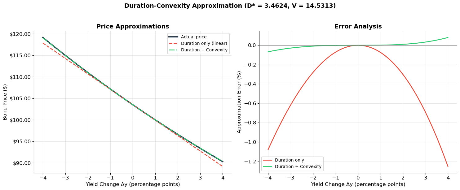

Yield move: 6% → 8% (+200 bps)
  Actual price:          $96.633628
  Duration approx:       $96.342094  (error: $0.291533)
  Duration+Convexity:    $96.642921  (error: $0.009294)
  Convexity reduces error by 31×

5. Immunization and Hedging¶

Duration Matching (Immunization)¶

A key application of duration is immunization: constructing a portfolio whose value is insensitive to small parallel shifts in the yield curve.

Goal: You have a liability due in $T$ years and want to invest in bonds such that the portfolio is protected against interest rate changes.

Strategy: Match the modified duration of assets to the modified duration of liabilities.

If you hold a bond portfolio with value $P_A$ and modified duration $D^*_A$ , and want to hedge a liability with value $P_L$ and modified duration $D^*_L$ :

\boxed{P_A \times D^*_A = P_L \times D^*_L}

(10)

This ensures that for small yield changes, the change in asset value offsets the change in liability value.

Hedging with a Different Bond¶

Suppose you are long a 4-year bond and want to hedge using 3-year bonds. You need:

\delta = -\frac{D^*_4 \times P_4}{D^*_3 \times P_3}

(11)

The hedge ratio $\delta$ tells you how many dollars of the 3-year bond to short per dollar of the 4-year bond.

Limitations¶

Duration matching only works for small, parallel yield curve shifts
The hedge must be rebalanced as time passes and yields change
For large or non-parallel shifts, convexity matching provides additional protection

# ============================================================
# Immunization Example
# ============================================================
# Pension fund has a $10M liability due in 7 years.
# Available instruments: 3-year and 10-year zero-coupon bonds, both yielding 5%.

# ▶ MODIFY AND RE-RUN
liability_pv = 10_000_000
liability_duration = 7.0
ytm_market = 0.05
T_short = 3
T_long = 10
# ============================================================

# Zero-coupon durations = maturity
D_short = T_short
D_long = T_long

# Weights: w * D_short + (1-w) * D_long = liability_duration
w_short = (D_long - liability_duration) / (D_long - D_short)
w_long = 1 - w_short

invest_short = liability_pv * w_short
invest_long = liability_pv * w_long

print("=" * 60)
print("IMMUNIZATION — Pension Fund Liability Matching")
print("=" * 60)
print(f"Liability PV:         ${liability_pv:>12,.0f}")
print(f"Liability duration:   {liability_duration:>12.1f} years")
print(f"\nAvailable instruments:")
print(f"  {T_short}-year zero (D = {D_short}):  weight = {w_short:.2%}")
print(f"  {T_long}-year zero (D = {D_long}): weight = {w_long:.2%}")
print(f"\nPortfolio allocation:")
print(f"  {T_short}-year zeros:  ${invest_short:>12,.0f}")
print(f"  {T_long}-year zeros: ${invest_long:>12,.0f}")
print(f"  Total invested: ${invest_short + invest_long:>12,.0f}")
print(f"  Portfolio D:    {w_short * D_short + w_long * D_long:.1f} years ✓")

# Test: yield shifts up 100bp — are we hedged?
yields_test = np.linspace(0.02, 0.08, 100)
port_values = []
liab_values = []

for y in yields_test:
    p_short = invest_short / (1 + ytm_market)**T_short * (1 + ytm_market)**T_short / (1 + y)**T_short
    p_long = invest_long / (1 + ytm_market)**T_long * (1 + ytm_market)**T_long / (1 + y)**T_long
    port_values.append(p_short + p_long)
    
    # Liability also reprices
    liab_fv = liability_pv * (1 + ytm_market)**liability_duration  # FV at maturity
    liab_values.append(liab_fv / (1 + y)**liability_duration)

fig, ax = plt.subplots(figsize=(11, 6))
ax.plot(yields_test * 100, np.array(port_values) / 1e6, color='#3498db', linewidth=2.5, label='Asset Portfolio')
ax.plot(yields_test * 100, np.array(liab_values) / 1e6, color='#e74c3c', linewidth=2.5, linestyle='--', label='Liability')
ax.axvline(x=ytm_market * 100, color='gray', linewidth=1, linestyle=':', alpha=0.5)
ax.set_xlabel('Yield (%)', fontsize=12)
ax.set_ylabel('Value ($M)', fontsize=12)
ax.set_title('Immunization: Assets Track Liability Under Yield Changes', fontsize=14, fontweight='bold')
ax.legend(fontsize=12)
ax.yaxis.set_major_formatter(mticker.FuncFormatter(lambda x, _: f'${x:.1f}M'))

plt.tight_layout()
plt.show()

print("The portfolio value closely tracks the liability for small yield shifts.")
print("This is duration matching (immunization) in action.")

============================================================
IMMUNIZATION — Pension Fund Liability Matching
============================================================
Liability PV:         $  10,000,000
Liability duration:            7.0 years

Available instruments:
  3-year zero (D = 3):  weight = 42.86%
  10-year zero (D = 10): weight = 57.14%

Portfolio allocation:
  3-year zeros:  $   4,285,714
  10-year zeros: $   5,714,286
  Total invested: $  10,000,000
  Portfolio D:    7.0 years ✓

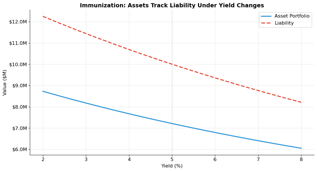
The portfolio value closely tracks the liability for small yield shifts.
This is duration matching (immunization) in action.

6. Corporate Bonds and Default Risk¶

Beyond Government Bonds¶

Government bonds are (approximately) riskless — the government can always print money to pay nominal obligations. Corporate bonds carry default risk: the issuer may fail to make promised payments.

Credit Ratings¶

Rating agencies (Moody’s, S&P, Fitch) assess default likelihood:

Grade	Moody’s	S&P	Description
Investment Grade
Highest	Aaa	AAA	Extremely strong
High	Aa	AA	Very strong
Upper Medium	A	A	Strong
Medium	Baa	BBB	Adequate (lowest IG)
Speculative (Junk)
Somewhat	Ba	BB	Speculative elements
Speculative	B	B	More vulnerable
Highly	Caa	CCC	Currently vulnerable
Default	C/D	D	In default

The dividing line between investment grade and speculative (Baa/BBB) is critical — many institutional investors (pension funds, insurance companies) are restricted to investment grade.

Yield Decomposition¶

Lo decomposes a corporate bond yield into components:

\boxed{y_{\text{corporate}} = y_{\text{risk-free}} + \underbrace{\text{Default Premium}}_{\text{expected loss}} + \underbrace{\text{Risk Premium}}_{\text{compensation for risk}} + \text{Liquidity, Tax, etc.}}

(12)

Promised YTM: the yield if default does not occur
Expected YTM: probability-weighted average of all outcomes
Default premium = Promised YTM − Expected YTM
Risk premium = Expected YTM − Risk-free YTM

# ============================================================
# Lo's Corporate Bond Yield Decomposition Example
# ============================================================
# From slide 47-48: 10-year zeros
# Treasury STRIPS: Price = $463.19, Face = $1,000
# XYZ Corp zero: Price = $321.97, Face = $1,000
# Expected payoff of XYZ: $762.22

F = 1000
P_treasury = 463.19
P_xyz = 321.97
E_payoff_xyz = 762.22
T = 10

# Yields
y_riskfree = (F / P_treasury)**(1/T) - 1
y_promised = (F / P_xyz)**(1/T) - 1
y_expected = (E_payoff_xyz / P_xyz)**(1/T) - 1

# Decomposition
default_premium = y_promised - y_expected
risk_premium = y_expected - y_riskfree

print("=" * 60)
print("CORPORATE BOND YIELD DECOMPOSITION — Lo's Example")
print("=" * 60)
print(f"10-Year Treasury STRIPS:  P = ${P_treasury:.2f},  YTM = {y_riskfree:.4%}")
print(f"10-Year XYZ Corp Zero:    P = ${P_xyz:.2f},  Face = ${F:,.0f}")
print(f"Expected payoff (XYZ):    ${E_payoff_xyz:.2f}")
print()
print(f"{'Component':>20s} {'Yield':>10s}")
print("-" * 35)
print(f"{'Risk-free yield':>20s} {y_riskfree:>10.4%}")
print(f"{'+ Risk premium':>20s} {risk_premium:>+10.4%}")
print(f"{'= Expected YTM':>20s} {y_expected:>10.4%}")
print(f"{'+ Default premium':>20s} {default_premium:>+10.4%}")
print(f"{'= Promised YTM':>20s} {y_promised:>10.4%}")
print("-" * 35)
total_spread = y_promised - y_riskfree
print(f"{'Total Credit Spread':>20s} {total_spread:>10.4%}")
print(f"\nOf the {total_spread*10000:.0f}bp spread over Treasuries:")
print(f"  {default_premium/total_spread*100:.0f}% is default premium (expected loss)")
print(f"  {risk_premium/total_spread*100:.0f}% is risk premium (compensation for bearing risk)")

============================================================
CORPORATE BOND YIELD DECOMPOSITION — Lo's Example
============================================================
10-Year Treasury STRIPS:  P = $463.19,  YTM = 8.0001%
10-Year XYZ Corp Zero:    P = $321.97,  Face = $1,000
Expected payoff (XYZ):    $762.22

           Component      Yield
-----------------------------------
     Risk-free yield    8.0001%
      + Risk premium   +0.9999%
      = Expected YTM    9.0000%
   + Default premium   +3.0001%
      = Promised YTM   12.0001%
-----------------------------------
 Total Credit Spread    4.0000%

Of the 400bp spread over Treasuries:
  75% is default premium (expected loss)
  25% is risk premium (compensation for bearing risk)

# ============================================================
# Visualization: Credit Spreads and Yield Decomposition
# ============================================================
fig, (ax1, ax2) = plt.subplots(1, 2, figsize=(14, 6))

# Left: Yield decomposition bar chart
components = ['Risk-free\nYield', 'Risk\nPremium', 'Default\nPremium']
values = [y_riskfree * 100, risk_premium * 100, default_premium * 100]
colors = ['#3498db', '#e67e22', '#e74c3c']
bottom = 0
for comp, val, color in zip(components, values, colors):
    ax1.bar('XYZ Corp\n10yr Zero', val, bottom=bottom, color=color, alpha=0.85,
            edgecolor='white', label=f'{comp}: {val:.2f}%')
    ax1.text(0, bottom + val/2, f'{val:.2f}%', ha='center', va='center',
            fontsize=11, fontweight='bold', color='white')
    bottom += val

ax1.bar('Treasury\n10yr', y_riskfree * 100, color='#3498db', alpha=0.85, edgecolor='white')
ax1.text(1, y_riskfree * 100 / 2, f'{y_riskfree*100:.2f}%', ha='center', va='center',
        fontsize=11, fontweight='bold', color='white')

ax1.set_ylabel('Yield (%)', fontsize=12)
ax1.set_title('Corporate Bond Yield Decomposition', fontsize=14, fontweight='bold')
ax1.legend(fontsize=9, loc='upper right')

# Right: Historical credit spreads (stylized)
np.random.seed(42)
years = np.arange(1990, 2009)
base_spread = 1.5 + 0.3 * np.sin(np.linspace(0, 4*np.pi, len(years)))
crisis_bump = np.zeros(len(years))
crisis_bump[-3:] = [1.5, 3.0, 8.0]  # 2006-2008 crisis
spreads = base_spread + crisis_bump + np.random.normal(0, 0.15, len(years))
spreads = np.maximum(spreads, 0.5)

ax2.fill_between(years, 0, spreads, alpha=0.3, color='#e74c3c')
ax2.plot(years, spreads, color='#e74c3c', linewidth=2.5)
ax2.axhline(y=2.0, color='gray', linewidth=1, linestyle=':', alpha=0.5)
ax2.annotate('2008 Crisis:\nSpreads explode', xy=(2008, spreads[-1]),
            xytext=(2002, spreads[-1] * 0.85),
            fontsize=11, color='#c0392b', fontweight='bold',
            arrowprops=dict(arrowstyle='->', color='#c0392b', lw=2))

ax2.set_xlabel('Year', fontsize=12)
ax2.set_ylabel('Baa − Treasury Spread (percentage points)', fontsize=12)
ax2.set_title('Corporate Credit Spreads Over Time\n(Stylized Baa − 10yr Treasury)', fontsize=14, fontweight='bold')
ax2.set_ylim(0)

plt.tight_layout()
plt.show()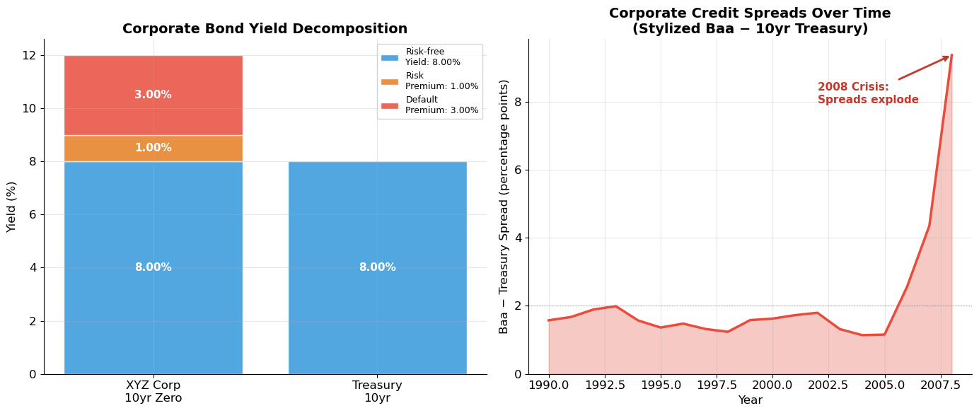

7. Securitization and the Sub-Prime Crisis¶

What Is Securitization?¶

Securitization takes a pool of risky assets (loans) and repackages them into tranches with different risk profiles. The idea is to create securities that are safer than the individual underlying loans.

Benefits (in theory):

Repackages risks into more homogeneous categories
More efficient allocation of risk across different investor types
Creates additional risk-bearing capacity
Provides transparency and supports economic growth

Requirements for success:

Diversification across loans
Accurate risk measurement
Normal market conditions (no systemic shocks)
Reasonably sophisticated investors

Lo’s Two-Bond CDO Example¶

This is one of the most important examples in the course. Lo strips the CDO mechanism to its bare essence to reveal the hidden role of correlation.

Setup:

Two identical 1-year bonds, each with $1,000 face value
Each bond defaults with probability 10% (pays $0) or pays off with probability 90% (pays $1,000)
Price of each bond = 0.9 × $1,000 + 0.1 × $0 = $900

Step 1: Pool them together. Create a portfolio of both bonds.

Step 2: Tranche them. Issue two new claims on the portfolio:

Senior tranche ($1,000): gets paid first
Junior tranche ($1,000): gets whatever is left

The key question: what are the tranches worth? It depends entirely on the correlation of defaults.

# ============================================================
# Lo's CDO Example: Independent Defaults
# ============================================================
face_per_bond = 1000
prob_default = 0.10
prob_pay = 1 - prob_default
n_bonds = 2

# Individual bond pricing
bond_price = prob_pay * face_per_bond + prob_default * 0
print("=" * 70)
print("Lo's CDO EXAMPLE — Two-Bond Securitization")
print("=" * 70)
print(f"Each bond: Face = ${face_per_bond:,}, Default prob = {prob_default:.0%}")
print(f"Each bond price: {prob_pay:.0%} × ${face_per_bond:,} + {prob_default:.0%} × $0 = ${bond_price:,.0f}")

# CASE 1: INDEPENDENT DEFAULTS
print("\n" + "=" * 70)
print("CASE 1: INDEPENDENT DEFAULTS")
print("=" * 70)

# Joint probabilities
p_both_pay = prob_pay ** 2             # 81%
p_one_defaults = 2 * prob_pay * prob_default  # 18%
p_both_default = prob_default ** 2     # 1%

states = [
    ('Both pay ($2,000)',    p_both_pay,      2000, 1000, 1000),
    ('One defaults ($1,000)', p_one_defaults, 1000, 1000, 0),
    ('Both default ($0)',    p_both_default,  0,    0,    0),
]

print(f"\n{'State':>25s} {'Prob':>8s} {'Portfolio':>12s} {'Senior':>10s} {'Junior':>10s}")
print("-" * 70)
senior_ev = 0
junior_ev = 0
for name, prob, port, sen, jun in states:
    print(f"{name:>25s} {prob:>8.0%} {port:>12,} {sen:>10,} {jun:>10,}")
    senior_ev += prob * sen
    junior_ev += prob * jun

print("-" * 70)
print(f"{'Expected Value':>25s} {'':>8s} {'$'+f'{senior_ev+junior_ev:,.0f}':>12s} {'$'+f'{senior_ev:,.0f}':>10s} {'$'+f'{junior_ev:,.0f}':>10s}")

# Default probabilities of tranches
senior_default_prob = p_both_default
junior_default_prob = p_one_defaults + p_both_default

print(f"\nSenior tranche: default prob = {senior_default_prob:.0%}  (was 10% per individual bond!)")
print(f"Junior tranche: default prob = {junior_default_prob:.0%}  (higher than individual)")
print(f"\n→ Diversification + tranching turned a 10%-default bond into a")
print(f"  Senior tranche with only {senior_default_prob:.0%} default probability — AAA territory!")

======================================================================
Lo's CDO EXAMPLE — Two-Bond Securitization
======================================================================
Each bond: Face = $1,000, Default prob = 10%
Each bond price: 90% × $1,000 + 10% × $0 = $900

======================================================================
CASE 1: INDEPENDENT DEFAULTS
======================================================================

                    State     Prob    Portfolio     Senior     Junior
----------------------------------------------------------------------
        Both pay ($2,000)      81%        2,000      1,000      1,000
    One defaults ($1,000)      18%        1,000      1,000          0
        Both default ($0)       1%            0          0          0
----------------------------------------------------------------------
           Expected Value                $1,800       $990       $810

Senior tranche: default prob = 1%  (was 10% per individual bond!)
Junior tranche: default prob = 19%  (higher than individual)

→ Diversification + tranching turned a 10%-default bond into a
  Senior tranche with only 1% default probability — AAA territory!

# ============================================================
# CASE 2: PERFECTLY CORRELATED DEFAULTS
# ============================================================
print("=" * 70)
print("CASE 2: PERFECTLY CORRELATED DEFAULTS")
print("=" * 70)
print("If the bonds ALWAYS default together (or pay together):")

states_corr = [
    ('Both pay ($2,000)',    prob_pay,     2000, 1000, 1000),
    ('Both default ($0)',    prob_default, 0,    0,    0),
]

print(f"\n{'State':>25s} {'Prob':>8s} {'Portfolio':>12s} {'Senior':>10s} {'Junior':>10s}")
print("-" * 70)
senior_ev_corr = 0
junior_ev_corr = 0
for name, prob, port, sen, jun in states_corr:
    print(f"{name:>25s} {prob:>8.0%} {port:>12,} {sen:>10,} {jun:>10,}")
    senior_ev_corr += prob * sen
    junior_ev_corr += prob * jun

print("-" * 70)
print(f"{'Expected Value':>25s} {'':>8s} {'$'+f'{senior_ev_corr+junior_ev_corr:,.0f}':>12s} {'$'+f'{senior_ev_corr:,.0f}':>10s} {'$'+f'{junior_ev_corr:,.0f}':>10s}")

print(f"\nSenior default prob: {prob_default:.0%}  (same as an individual bond!)")
print(f"Junior default prob: {prob_default:.0%}  (also same — correlation destroys diversification)")

print("\n" + "=" * 70)
print("COMPARISON: THE DEVASTATING EFFECT OF CORRELATION")
print("=" * 70)
print(f"{'':>25s} {'Independent':>15s} {'Correlated':>15s} {'Change':>12s}")
print("-" * 70)
print(f"{'Senior price':>25s} {'$'+f'{senior_ev:,.0f}':>15s} {'$'+f'{senior_ev_corr:,.0f}':>15s} {'$'+f'{senior_ev_corr - senior_ev:+,.0f}':>12s}")
print(f"{'Junior price':>25s} {'$'+f'{junior_ev:,.0f}':>15s} {'$'+f'{junior_ev_corr:,.0f}':>15s} {'$'+f'{junior_ev_corr - junior_ev:+,.0f}':>12s}")
print(f"{'Senior default prob':>25s} {senior_default_prob:>15.0%} {prob_default:>15.0%} {'10× worse!':>12s}")
print(f"\n→ The senior tranche goes from near-riskless (1% default)")
print(f"  to as risky as a single bond (10% default) — a TEN-FOLD increase!")
print(f"  This is EXACTLY what happened in the 2008 financial crisis.")

======================================================================
CASE 2: PERFECTLY CORRELATED DEFAULTS
======================================================================
If the bonds ALWAYS default together (or pay together):

                    State     Prob    Portfolio     Senior     Junior
----------------------------------------------------------------------
        Both pay ($2,000)      90%        2,000      1,000      1,000
        Both default ($0)      10%            0          0          0
----------------------------------------------------------------------
           Expected Value                $1,800       $900       $900

Senior default prob: 10%  (same as an individual bond!)
Junior default prob: 10%  (also same — correlation destroys diversification)

======================================================================
COMPARISON: THE DEVASTATING EFFECT OF CORRELATION
======================================================================
                              Independent      Correlated       Change
----------------------------------------------------------------------
             Senior price            $990            $900         $-90
             Junior price            $810            $900         $+90
      Senior default prob              1%             10%   10× worse!

→ The senior tranche goes from near-riskless (1% default)
  to as risky as a single bond (10% default) — a TEN-FOLD increase!
  This is EXACTLY what happened in the 2008 financial crisis.

# ============================================================
# Visualization: CDO Tranche Values vs. Correlation
# ============================================================
# Generalize: vary correlation from 0 (independent) to 1 (perfectly correlated)
# Using a simple bivariate model with mixing parameter rho

rho_range = np.linspace(0, 1, 100)
senior_prices = []
junior_prices = []
senior_def_probs = []

for rho in rho_range:
    # Joint default probability with correlation rho
    # P(both default) = rho * p + (1-rho) * p^2
    p_both_def = rho * prob_default + (1 - rho) * prob_default**2
    # P(exactly one defaults) = 2*p*(1-p) * (1-rho)
    p_one_def = (1 - rho) * 2 * prob_default * prob_pay
    # P(both pay) = 1 - p_both_def - p_one_def
    p_both_pay_rho = 1 - p_both_def - p_one_def
    
    # Senior gets $1000 unless both default
    s_price = (p_both_pay_rho + p_one_def) * 1000
    # Junior gets $1000 only if both pay
    j_price = p_both_pay_rho * 1000
    
    senior_prices.append(s_price)
    junior_prices.append(j_price)
    senior_def_probs.append(p_both_def * 100)

fig, (ax1, ax2) = plt.subplots(1, 2, figsize=(14, 6))

# Left: Tranche prices vs correlation
ax1.plot(rho_range, senior_prices, color='#3498db', linewidth=3, label='Senior Tranche')
ax1.plot(rho_range, junior_prices, color='#e74c3c', linewidth=3, label='Junior Tranche')
ax1.axhline(y=900, color='gray', linewidth=1, linestyle=':', alpha=0.5, label='Individual bond ($900)')

ax1.set_xlabel('Default Correlation (ρ)', fontsize=13)
ax1.set_ylabel('Tranche Value ($)', fontsize=13)
ax1.set_title('Tranche Values vs. Default Correlation', fontsize=14, fontweight='bold')
ax1.legend(fontsize=11)
ax1.yaxis.set_major_formatter(mticker.FuncFormatter(lambda x, _: f'${x:,.0f}'))

# Key points
ax1.annotate(f'Independent:\nSenior = ${senior_prices[0]:,.0f}', xy=(0, senior_prices[0]),
            xytext=(0.15, senior_prices[0] + 10), fontsize=9, color='#3498db',
            arrowprops=dict(arrowstyle='->', color='#3498db'))
ax1.annotate(f'Correlated:\nSenior = ${senior_prices[-1]:,.0f}', xy=(1, senior_prices[-1]),
            xytext=(0.7, senior_prices[-1] + 30), fontsize=9, color='#3498db',
            arrowprops=dict(arrowstyle='->', color='#3498db'))

# Right: Senior default probability vs correlation
ax2.plot(rho_range, senior_def_probs, color='#e74c3c', linewidth=3)
ax2.fill_between(rho_range, 0, senior_def_probs, alpha=0.15, color='#e74c3c')
ax2.axhline(y=1, color='#2ecc71', linewidth=1.5, linestyle='--', alpha=0.7, label='Independent: 1%')
ax2.axhline(y=10, color='#e74c3c', linewidth=1.5, linestyle='--', alpha=0.7, label='Correlated: 10%')

ax2.set_xlabel('Default Correlation (ρ)', fontsize=13)
ax2.set_ylabel('Senior Default Probability (%)', fontsize=13)
ax2.set_title('Senior Tranche Default Risk\nvs. Correlation', fontsize=14, fontweight='bold')
ax2.legend(fontsize=10)

fig.suptitle("The Sub-Prime Mechanism: How Correlation Destroys 'Safe' Assets",
             fontsize=15, fontweight='bold', y=1.03)
plt.tight_layout()
plt.show()

print("This is the sub-prime crisis in one graph:")
print("• Rating agencies assumed low correlation → AAA rating for senior tranches")
print("• When housing markets declined NATIONALLY, correlations spiked toward 1")
print("• 'AAA' tranches suffered default rates 10× higher than rated")
print("• Institutions holding these 'safe' assets faced catastrophic losses")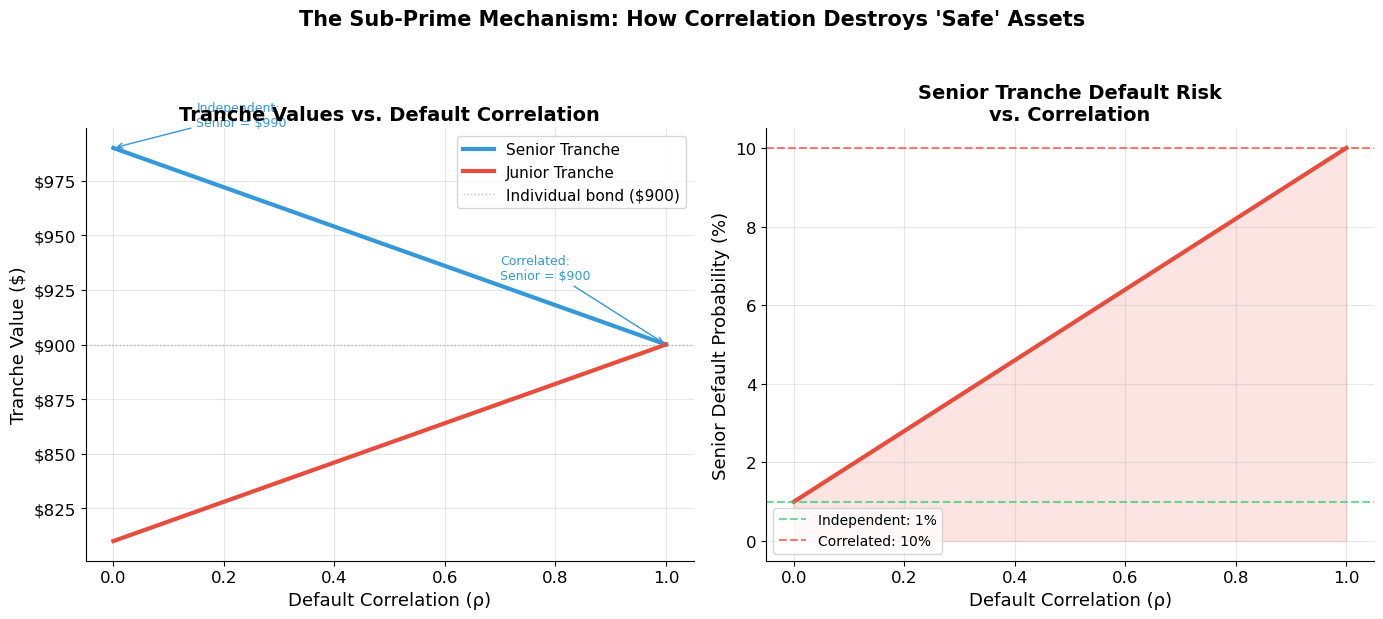

This is the sub-prime crisis in one graph:
• Rating agencies assumed low correlation → AAA rating for senior tranches
• When housing markets declined NATIONALLY, correlations spiked toward 1
• 'AAA' tranches suffered default rates 10× higher than rated
• Institutions holding these 'safe' assets faced catastrophic losses

The Sub-Prime Narrative (Lo’s Real-Time Account)¶

Lo connects the CDO mechanism to the actual crisis timeline:

Pre-2007: Very low default rates on mortgages. Very low correlation of defaults (regional, not national). Senior tranches correctly rated AAA under these assumptions. Enormous demand: pension funds bought senior tranches (safe yield), hedge funds bought junior tranches (high yield).
2007–2008: National real-estate market declines for the first time in decades. Default correlation rises dramatically — when one borrower defaults, nearby borrowers are also likely to default (falling house prices affect entire neighborhoods, cities, states).
Consequence: Senior tranches that were rated AAA with ~1% default probability suddenly face default rates of 10% or higher. Ratings agencies downgrade massively. Institutions that could only hold investment-grade bonds are forced to sell.
Cascade: Forced selling → further price declines → more defaults → more downgrades → more forced selling. This is the death spiral that brought down Lehman Brothers, Bear Stearns, AIG, and nearly the entire global financial system.

The key lesson: securitization works brilliantly when defaults are independent, and catastrophically when they become correlated. The model assumption of low correlation was the fatal flaw.

8. Exercises¶

Exercise 1: Duration and Price Sensitivity¶

A 10-year bond has a face value of $1,000, a 6% annual coupon, and is priced to yield 5%.

(a) Compute the Macaulay duration and modified duration.

(b) If yields rise by 50 basis points, estimate the percentage price change using duration. Compare with the actual price change.

(c) Now add convexity. Compute the bond’s convexity and re-estimate the price change. How much does the convexity correction improve the approximation?

(d) Repeat parts (b)–(c) for a 200bp yield increase. When does convexity become essential?

# Exercise 1 — Workspace
# face, coupon_rate, maturity, ytm = 1000, 0.06, 10, 0.05
# P = bond_price_from_ytm(face, coupon_rate, maturity, ytm)
# D = macaulay_duration(face, coupon_rate, maturity, ytm)
# Dmod = modified_duration(face, coupon_rate, maturity, ytm)
# V = bond_convexity(face, coupon_rate, maturity, ytm)
# print(f"Price: ${P:,.2f}")
# print(f"Macaulay D: {D:.4f}")
# print(f"Modified D: {Dmod:.4f}")
# print(f"Convexity:  {V:.4f}")
#
# for dy in [0.005, 0.02]:
#     actual = bond_price_from_ytm(face, coupon_rate, maturity, ytm+dy)
#     dur_est = P * (1 - Dmod * dy)
#     dc_est = P * (1 - Dmod * dy + 0.5 * V * dy**2)
#     print(f"\nΔy = {dy*10000:.0f}bp:")
#     print(f"  Actual:  ${actual:,.2f}  ({(actual/P-1)*100:+.4f}%)")
#     print(f"  Dur:     ${dur_est:,.2f}  (error: ${abs(dur_est-actual):,.2f})")
#     print(f"  Dur+Conv:${dc_est:,.2f}  (error: ${abs(dc_est-actual):,.2f})")

Exercise 2: Immunization¶

You manage a pension fund with a $50M liability due in 8 years. Yields are currently 4% across all maturities. You can invest in:

Bond A: 5-year, 3% annual coupon, $1,000 par
Bond B: 15-year, 5% annual coupon, $1,000 par

(a) Compute the price, Macaulay duration, and modified duration of each bond.

(b) What portfolio weights (in Bonds A and B) immunize the liability?

(c) If yields jump to 5%, calculate the change in portfolio value and liability value. Is the portfolio still approximately hedged?

(d) Why might you prefer to use zero-coupon bonds for immunization instead of coupon bonds? What are the trade-offs?

# Exercise 2 — Workspace
# y = 0.04
# PA = bond_price_from_ytm(1000, 0.03, 5, y)
# PB = bond_price_from_ytm(1000, 0.05, 15, y)
# DA = macaulay_duration(1000, 0.03, 5, y)
# DB = macaulay_duration(1000, 0.05, 15, y)
# print(f"Bond A: P=${PA:,.2f}, D={DA:.4f}")
# print(f"Bond B: P=${PB:,.2f}, D={DB:.4f}")
#
# # Target duration = 8
# w_A = (DB - 8) / (DB - DA)
# w_B = 1 - w_A
# print(f"Weights: A={w_A:.4f}, B={w_B:.4f}")
# print(f"Portfolio D: {w_A*DA + w_B*DB:.4f}")

Exercise 3: Securitization and Correlation¶

Consider a pool of three identical 1-year bonds, each with:

Face value: $1,000
Default probability: 5%
Defaults are independent

The pool is tranched into: Senior ($1,000), Mezzanine ($1,000), Equity ($1,000).

(a) List all possible portfolio outcomes and their probabilities.

(b) Compute the expected payoff, price, and default probability for each tranche. Show that the senior tranche has a very low default probability.

(c) Now assume defaults are perfectly correlated. Recompute all tranche values and default probabilities. What happens to the senior tranche?

(d) Consider an intermediate case: 50% correlation (half the time defaults are independent, half the time they’re perfectly correlated). Compute tranche values. How sensitive are the results to the correlation assumption?

(e) Discuss: why did rating agencies get this so wrong? What institutional incentives were at play?

# Exercise 3 — Workspace
# p_d = 0.05
# p_p = 0.95
#
# # Independent: 3 bonds, binomial distribution
# # k defaults out of 3:
# from math import comb
# for k in range(4):
#     prob = comb(3, k) * p_d**k * p_p**(3-k)
#     portfolio_val = (3-k) * 1000
#     senior = min(portfolio_val, 1000)
#     mezz = min(max(portfolio_val - 1000, 0), 1000)
#     equity = max(portfolio_val - 2000, 0)
#     print(f"k={k} defaults: prob={prob:.6f}, portfolio=${portfolio_val:,}, "
#           f"senior=${senior:,}, mezz=${mezz:,}, equity=${equity:,}")

Key Takeaways — Session 5¶

Macaulay duration is the PV-weighted average time to receipt of cash flows. It measures bond “effective maturity.”
Modified duration $D^* = D/(1+y/q)$ gives the percentage price sensitivity: $\Delta P/P \approx -D^* \times \Delta y$ . It is the single most important number in fixed-income risk management.
Convexity captures curvature. The duration-convexity approximation $\Delta P/P \approx -D^* \Delta y + \frac{1}{2} V (\Delta y)^2$ is essential for large yield movements.
Immunization (duration matching) protects portfolios against small parallel yield shifts. It requires continuous rebalancing.
Corporate bond yields decompose into risk-free rate + default premium + risk premium + other factors.
Securitization creates tranches with different risk profiles from a pool of assets. Diversification across loans makes senior tranches very safe — but only if defaults are independent.
The 2008 crisis was fundamentally a correlation event: when housing markets declined nationally, default correlations spiked, AAA tranches suffered massive losses, and the “safe” became toxic.

References¶

Brealey, R.A., Myers, S.C., and Allen, F. Principles of Corporate Finance, Chapters 23–25.
MIT OCW 15.401: Fixed-Income Securities
Macaulay, F. (1938). Some Theoretical Problems Suggested by the Movements of Interest Rates, Bond Yields and Stock Prices in the United States since 1856. NBER.
Sundaresan, S. (1997). Fixed Income Markets and Their Derivatives. South-Western.
Lo, A.W. (2012). “Reading about the Financial Crisis: A Twenty-One Book Review.” Journal of Economic Literature, 50(1), 151–178.

Next: Session 6 — Equities — stock valuation, the dividend discount model, earnings multiples, and the price-to-earnings ratio.