Lecture 4: Fixed-Income Securities I — Bond Pricing, Spot Rates, and the Term Structure
MIT 15.401 — Finance Theory I (Prof. Andrew Lo)
Video: MIT OCW — Part I & II of Fixed-Income Securities
Readings: Brealey, Myers, and Allen — Chapters 23–25; Sundaresan, Fixed Income Markets and Their Derivatives
This notebook begins the Fixed-Income Securities block (Sessions 4–7), which applies the present value machinery to the largest asset class in the world. The US bond market alone exceeded $26 trillion in outstanding debt in 2006 — dwarfing the equity market.
Session 4 covers the foundations: what fixed-income securities are, how to price discount (zero-coupon) bonds, the concept of spot rates and the term structure of interest rates, how to extract forward rates from the yield curve, and how to value coupon bonds using both spot rates and the yield-to-maturity (YTM) convention.
This lecture is heavy on notation but light on new conceptual challenges — everything builds on the NPV framework from Sessions 2–3. The key new insight is that the yield curve embeds the market’s expectations about future interest rates.
Table of Contents
Source
# ============================================================
# Setup
# ============================================================
import numpy as np
import pandas as pd
import matplotlib.pyplot as plt
import matplotlib.ticker as mticker
from scipy.optimize import brentq
from IPython.display import display, Markdown

plt.rcParams.update({
    'figure.figsize': (10, 5),
    'axes.spines.top': False,
    'axes.spines.right': False,
    'axes.grid': True,
    'grid.alpha': 0.3,
    'font.size': 12,
    'lines.linewidth': 2,
})

print("Libraries loaded successfully.")
Libraries loaded successfully.
1. Industry Overview — The Bond Market
What Are Fixed-Income Securities?
Fixed-income securities are financial claims with promised cash flows of known fixed amount paid at fixed dates. The key word is promised — the cash flows are contractually specified, unlike equities where dividends are uncertain.
Classification
| Category | Examples |
|---|---|
| Treasury Securities | US T-bills (< 1 year), T-notes (1–10 years), T-bonds (10–30 years) |
| Federal Agency | FNMA (Fannie Mae), FHLMC (Freddie Mac), GNMA (Ginnie Mae) |
| Corporate | Commercial paper, medium-term notes (MTNs), corporate bonds |
| Municipal | State and local government bonds (often tax-exempt) |
| Mortgage-Backed | Pass-throughs, CMOs, RMBS, CMBS |
| Asset-Backed | Securities backed by auto loans, credit cards, student loans |
| Derivatives | CDOs, CDS, interest rate swaps |
Market Scale
The US bond market in 2006 (Lo’s data): $26.7 trillion outstanding — roughly split as mortgage-related (24%), corporate (19%), Treasury (16%), money markets (14%), federal agency (10%), municipal (9%), and asset-backed (8%).
Market Participants
Issuers: Governments, corporations, banks, municipalities, SPVs, foreign institutions. Intermediaries: Primary dealers, investment banks, rating agencies (Moody’s, S&P, Fitch). Investors: Pension funds, insurance companies, mutual funds, hedge funds, central banks, individuals.
Source
# ============================================================
# US Bond Market Composition (Lo's 2006 data)
# ============================================================
categories = ['Mortgage-\nRelated', 'Corporate', 'Treasury', 'Money\nMarkets',
              'Federal\nAgency', 'Municipal', 'Asset-\nBacked']
outstanding = [6400.4, 5209.7, 4283.8, 3818.9, 2665.2, 2337.5, 2016.7]
colors = ['#e74c3c', '#3498db', '#2c3e50', '#95a5a6', '#e67e22', '#2ecc71', '#9b59b6']

fig, (ax1, ax2) = plt.subplots(1, 2, figsize=(14, 6))

# Pie chart
wedges, texts, autotexts = ax1.pie(outstanding, labels=categories, autopct='%1.0f%%',
                                    colors=colors, startangle=90, pctdistance=0.75)
for t in autotexts:
    t.set_fontsize(10)
    t.set_fontweight('bold')
ax1.set_title('US Bond Market Outstanding\n($26.7 Trillion, 2006)', fontsize=14, fontweight='bold')

# Bar chart
sorted_idx = np.argsort(outstanding)[::-1]
sorted_cats = [categories[i] for i in sorted_idx]
sorted_vals = [outstanding[i] for i in sorted_idx]
sorted_colors = [colors[i] for i in sorted_idx]
bars = ax2.barh(sorted_cats, sorted_vals, color=sorted_colors, alpha=0.85, edgecolor='white')
ax2.set_xlabel('Outstanding ($Billions)')
ax2.set_title('Bond Market by Segment', fontsize=14, fontweight='bold')
ax2.invert_yaxis()
for bar, val in zip(bars, sorted_vals):
    ax2.text(val + 100, bar.get_y() + bar.get_height()/2,
            f'${val:,.0f}B', va='center', fontsize=10)

plt.tight_layout()
plt.show()

total = sum(outstanding)
print(f"Total US bond market: ${total:,.1f} billion = ${total/1000:.1f} trillion")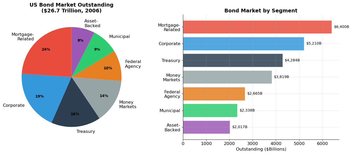
Total US bond market: $26,732.2 billion = $26.7 trillion
2. Valuation of Discount (Zero-Coupon) Bonds
Definition
A pure discount bond (or zero-coupon bond) pays a single cash flow — the face value — at maturity date . There are no intermediate coupon payments.
Examples: US Treasury bills (maturities < 1 year) and STRIPS (Separate Trading of Registered Interest and Principal Securities, maturities up to 30 years).
Pricing
The price of a discount bond is simply the present value of its face value:
where is the spot rate — the annualized yield for lending from today (time 0) to time .
Note that form a system of three variables with one equation — given any two, the third is determined. In particular, from observed prices we can extract spot rates:
Lo’s STRIPS Example (August 1, 2001)
| Maturity | Price (per $1 face) | Implied Spot Rate |
|---|---|---|
| 3 months | 0.991 | — |
| 6 months | 0.983 | — |
| 1 year | 0.967 | 3.41% |
| 2 years | 0.927 | 3.82% |
| 5 years | 0.797 | 4.64% |
| 10 years | 0.605 | 5.15% |
| 30 years | 0.187 | 5.64% |
Source
# ============================================================
# STRIPS Pricing and Spot Rate Extraction
# ============================================================
strips_data = {
    0.25: 0.991,
    0.50: 0.983,
    1:    0.967,
    2:    0.927,
    5:    0.797,
    10:   0.605,
    30:   0.187,
}

print("=" * 65)
print("STRIPS PRICES AND IMPLIED SPOT RATES (August 1, 2001)")
print("=" * 65)
print(f"{'Maturity':>10s} {'Price':>10s} {'Spot Rate':>12s} {'Discount Factor':>16s}")
print("-" * 65)

maturities, spot_rates, prices = [], [], []
for T, P in strips_data.items():
    r = (1 / P)**(1 / T) - 1
    maturities.append(T)
    spot_rates.append(r)
    prices.append(P)
    print(f"{T:>10.2f} {P:>10.3f} {r:>12.4%} {P:>16.4f}")

fig, (ax1, ax2) = plt.subplots(1, 2, figsize=(14, 6))

# Left: Discount bond prices
ax1.plot(maturities, prices, 'o-', color='#3498db', linewidth=2.5, markersize=8)
ax1.set_xlabel('Maturity (Years)', fontsize=12)
ax1.set_ylabel('Price (per $1 Face)', fontsize=12)
ax1.set_title('STRIPS Prices', fontsize=14, fontweight='bold')
ax1.set_ylim(0, 1.05)
for m, p in zip(maturities, prices):
    ax1.annotate(f'${p:.3f}', xy=(m, p), xytext=(m + 0.5, p + 0.03), fontsize=9)

# Right: Term structure (spot rates)
ax2.plot(maturities, [r * 100 for r in spot_rates], 'o-', color='#e74c3c', linewidth=2.5, markersize=8)
ax2.set_xlabel('Maturity (Years)', fontsize=12)
ax2.set_ylabel('Spot Rate (%)', fontsize=12)
ax2.set_title('Term Structure of Interest Rates', fontsize=14, fontweight='bold')
for m, r in zip(maturities, spot_rates):
    ax2.annotate(f'{r:.2%}', xy=(m, r * 100), xytext=(m + 0.5, r * 100 + 0.05), fontsize=9)

plt.tight_layout()
plt.show()
=================================================================
STRIPS PRICES AND IMPLIED SPOT RATES (August 1, 2001)
=================================================================
Maturity Price Spot Rate Discount Factor
-----------------------------------------------------------------
0.25 0.991 3.6825% 0.9910
0.50 0.983 3.4887% 0.9830
1.00 0.967 3.4126% 0.9670
2.00 0.927 3.8628% 0.9270
5.00 0.797 4.6426% 0.7970
10.00 0.605 5.1537% 0.6050
30.00 0.187 5.7479% 0.1870
3. Spot Rates and the Term Structure
Notation
We need careful notation because interest rates now vary by maturity.
| Symbol | Meaning |
|---|---|
| Spot rate: today’s annualized rate for lending/borrowing from to | |
| Future one-period spot rate: the one-year rate that will prevail in year (unknown today) | |
| Forward rate: today’s rate for a one-year loan beginning in year (known today, implied by the term structure) | |
| or | Price today of a discount bond maturing at |
The Relationship Between Spot Rates and Future Rates
Today’s -year spot rate is a geometric average of future one-period rates:
But we don’t observe the future rates . What we do observe are spot rates from current bond prices.
The Term Structure
A plot of spot rates against maturity is the term structure of interest rates (or the spot rate curve). It encodes the market’s collective information about current and future interest rates.
Shapes of the term structure:
Normal (upward-sloping): long-term rates > short-term rates — most common
Flat: all rates approximately equal
Inverted: short-term rates > long-term rates — historically a recession predictor
Humped: rates rise then fall
Source
# ============================================================
# Term Structure Shapes — Illustrative Examples
# ============================================================
T = np.linspace(0.25, 30, 200)

# Four canonical shapes
normal = 2 + 2.5 * (1 - np.exp(-T / 5))
flat = np.ones_like(T) * 4.0
inverted = 5.5 - 2 * (1 - np.exp(-T / 3))
humped = 3 + 2 * T * np.exp(-T / 3)

fig, axes = plt.subplots(2, 2, figsize=(13, 9))
configs = [
    (axes[0, 0], normal, 'Normal (Upward-Sloping)', '#3498db',
     'Most common. Markets expect\nrising rates or demand a\nterm/liquidity premium.'),
    (axes[0, 1], flat, 'Flat', '#2ecc71',
     'Transition state. No expected\nchange in rates.'),
    (axes[1, 0], inverted, 'Inverted', '#e74c3c',
     'Short > long. Historically\nassociated with impending\nrecession.'),
    (axes[1, 1], humped, 'Humped', '#9b59b6',
     'Rates rise then fall.\nExpectation of rate changes\nat intermediate horizon.'),
]

for ax, curve, title, color, note in configs:
    ax.plot(T, curve, color=color, linewidth=3)
    ax.set_xlabel('Maturity (Years)', fontsize=10)
    ax.set_ylabel('Spot Rate (%)', fontsize=10)
    ax.set_title(title, fontsize=13, fontweight='bold', color=color)
    ax.set_xlim(0, 30)
    ax.text(0.95, 0.05, note, transform=ax.transAxes, ha='right', va='bottom',
            fontsize=9, style='italic', color='#555',
            bbox=dict(boxstyle='round,pad=0.4', facecolor='#f8f8f8', alpha=0.9))

fig.suptitle('Canonical Term Structure Shapes', fontsize=15, fontweight='bold', y=1.01)
plt.tight_layout()
plt.show()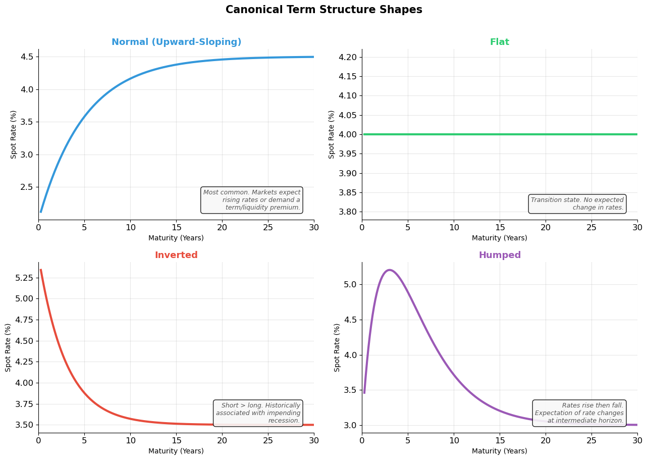
4. Forward Rates
Extracting Forward Rates from Spot Rates
The forward rate is the interest rate for a one-year loan beginning at time , as implied by today’s term structure. It is not a forecast — it is an arbitrage-free rate locked in by current prices.
From the no-arbitrage condition:
Solving for the forward rate:
Intuition: Investing for years at the -year spot rate must give the same return as investing for years at the -year spot rate and then reinvesting for one year at the forward rate . Otherwise, there’s an arbitrage.
Lo’s CFO Example
As the CFO of a US multinational, you expect to repatriate $10M from a foreign subsidiary in one year, which will be used to pay dividends one year later. You want to lock in a lending rate from year 1 to year 2.
Current rates: and
Strategy:
Borrow $9.524M for 1 year at 5% (creates $10M obligation at year 1)
Invest $9.524M for 2 years at 7% (grows to $10.904M at year 2)
At year 1, use the $10M repatriation to repay the 1-year loan
At year 2, collect $10.904M
Result: You’ve locked in a 1-year rate from year 1 to 2 of $10.904M/$10M - 1 = 9.04%. This is the forward rate .
Source
# ============================================================
# Forward Rate Extraction from Spot Rates
# ============================================================

def extract_forward_rates(maturities, spot_rates):
    """Extract 1-year forward rates from a set of spot rates.

    f_T = (1 + r_T)^T / (1 + r_{T-1})^{T-1} - 1
    """
    forwards = {}
    sorted_pairs = sorted(zip(maturities, spot_rates))

    for i in range(len(sorted_pairs)):
        T, r_T = sorted_pairs[i]
        if i == 0:
            forwards[T] = r_T  # First forward = first spot rate
        else:
            T_prev, r_prev = sorted_pairs[i - 1]
            if T - T_prev == 1:  # Only compute for integer-year gaps
                f = (1 + r_T)**T / (1 + r_prev)**T_prev - 1
                forwards[T] = f
    return forwards


# Example: Build a richer term structure for integer maturities
spot_rates_annual = {
    1: 0.0341,
    2: 0.0382,
    3: 0.0410,
    4: 0.0435,
    5: 0.0464,
    6: 0.0480,
    7: 0.0495,
    8: 0.0505,
    9: 0.0512,
    10: 0.0515,
}

forwards = extract_forward_rates(
    list(spot_rates_annual.keys()),
    list(spot_rates_annual.values())
)

print("=" * 65)
print("SPOT RATES AND IMPLIED FORWARD RATES")
print("=" * 65)
print(f"{'Maturity':>10s} {'Spot Rate':>12s} {'Forward Rate':>14s} {'Interpretation':>25s}")
print("-" * 65)
for T in sorted(spot_rates_annual.keys()):
    r = spot_rates_annual[T]
    f = forwards.get(T, None)
    if f is not None:
        interp = f"1yr rate in year {T}"
        print(f"{T:>10d} {r:>12.4%} {f:>14.4%} {interp:>25s}")

# Verify: compounding forward rates should recover spot rates
print("\n--- Verification: Forward rates compound to spot rates ---")
cumulative = 1.0
for T in range(1, 11):
    cumulative *= (1 + forwards[T])
    implied_spot = cumulative**(1/T) - 1
    actual_spot = spot_rates_annual[T]
    check = '✓' if abs(implied_spot - actual_spot) < 1e-10 else '✗'
    print(f"  T={T:>2d}: (1+f1)×...×(1+f{T})^(1/{T}) = {implied_spot:.4%} vs r_{T} = {actual_spot:.4%}  {check}")
=================================================================
SPOT RATES AND IMPLIED FORWARD RATES
=================================================================
Maturity Spot Rate Forward Rate Interpretation
-----------------------------------------------------------------
1 3.4100% 3.4100% 1yr rate in year 1
2 3.8200% 4.2316% 1yr rate in year 2
3 4.1000% 4.6623% 1yr rate in year 3
4 4.3500% 5.1036% 1yr rate in year 4
5 4.6400% 5.8081% 1yr rate in year 5
6 4.8000% 5.6037% 1yr rate in year 6
7 4.9500% 5.8545% 1yr rate in year 7
8 5.0500% 5.7527% 1yr rate in year 8
9 5.1200% 5.6817% 1yr rate in year 9
10 5.1500% 5.4204% 1yr rate in year 10
--- Verification: Forward rates compound to spot rates ---
T= 1: (1+f1)×...×(1+f1)^(1/1) = 3.4100% vs r_1 = 3.4100% ✓
T= 2: (1+f1)×...×(1+f2)^(1/2) = 3.8200% vs r_2 = 3.8200% ✓
T= 3: (1+f1)×...×(1+f3)^(1/3) = 4.1000% vs r_3 = 4.1000% ✓
T= 4: (1+f1)×...×(1+f4)^(1/4) = 4.3500% vs r_4 = 4.3500% ✓
T= 5: (1+f1)×...×(1+f5)^(1/5) = 4.6400% vs r_5 = 4.6400% ✓
T= 6: (1+f1)×...×(1+f6)^(1/6) = 4.8000% vs r_6 = 4.8000% ✓
T= 7: (1+f1)×...×(1+f7)^(1/7) = 4.9500% vs r_7 = 4.9500% ✓
T= 8: (1+f1)×...×(1+f8)^(1/8) = 5.0500% vs r_8 = 5.0500% ✓
T= 9: (1+f1)×...×(1+f9)^(1/9) = 5.1200% vs r_9 = 5.1200% ✓
T=10: (1+f1)×...×(1+f10)^(1/10) = 5.1500% vs r_10 = 5.1500% ✓
Source
# ============================================================
# Visualization: Spot Curve vs. Forward Curve
# ============================================================
T_vals = sorted(spot_rates_annual.keys())
spot_vals = [spot_rates_annual[T] * 100 for T in T_vals]
fwd_vals = [forwards[T] * 100 for T in T_vals]

fig, ax = plt.subplots(figsize=(12, 6))

ax.plot(T_vals, spot_vals, 'o-', color='#2c3e50', linewidth=3, markersize=8, label='Spot Rate Curve', zorder=3)
ax.plot(T_vals, fwd_vals, 's--', color='#e74c3c', linewidth=2, markersize=7, label='Forward Rate Curve', zorder=3)
ax.fill_between(T_vals, spot_vals, fwd_vals, alpha=0.1, color='#e74c3c')

ax.set_xlabel('Maturity / Forward Period (Years)', fontsize=13)
ax.set_ylabel('Rate (%)', fontsize=13)
ax.set_title('Spot Rates vs. Implied Forward Rates', fontsize=14, fontweight='bold')
ax.legend(fontsize=12, loc='lower right')

# Annotate key insight
ax.annotate('Forward curve lies ABOVE\nspot curve when term\nstructure is upward-sloping',
            xy=(7, fwd_vals[6]), xytext=(4, fwd_vals[6] + 0.8),
            fontsize=10, color='#e74c3c', style='italic',
            arrowprops=dict(arrowstyle='->', color='#e74c3c', lw=1.5),
            bbox=dict(boxstyle='round,pad=0.4', facecolor='#fdf2f2', alpha=0.9))

plt.tight_layout()
plt.show()

print("Key Insight: When the spot curve is upward-sloping, forward rates")
print("exceed spot rates. Intuitively, if long rates are higher than short")
print("rates, the 'marginal' rate for the next year must be even higher")
print("to pull up the average.")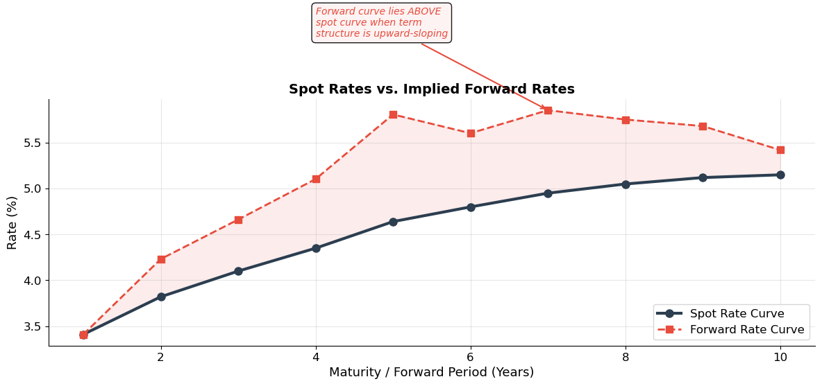
Key Insight: When the spot curve is upward-sloping, forward rates
exceed spot rates. Intuitively, if long rates are higher than short
rates, the 'marginal' rate for the next year must be even higher
to pull up the average.
Source
# ============================================================
# Lo's CFO Example: Locking in a Forward Rate
# ============================================================
r1 = 0.05   # 1-year spot rate
r2 = 0.07   # 2-year spot rate
repatriation = 10_000_000  # $10M arriving at year 1

# Implied forward rate
f2 = (1 + r2)**2 / (1 + r1) - 1

# Strategy
borrow_amount = repatriation / (1 + r1)  # Borrow this much at year 0
invest_amount = borrow_amount              # Invest same amount for 2 years
year2_proceeds = invest_amount * (1 + r2)**2
year1_repayment = repatriation

print("=" * 60)
print("CFO FORWARD RATE LOCK — Lo's Example")
print("=" * 60)
print(f"1-year spot rate:      {r1:.2%}")
print(f"2-year spot rate:      {r2:.2%}")
print(f"Implied forward rate:  {f2:.4%}")
print()

# Cash flow table
cf_data = {
    'Transaction': [
        'Borrow for 1 year at 5%',
        'Invest for 2 years at 7%',
        'Repatriation received',
        'Repay 1-year loan',
        'Collect 2-year investment',
        'NET'
    ],
    'Year 0': [
        f'+${borrow_amount:,.0f}', f'-${invest_amount:,.0f}', '—', '—', '—', '$0'
    ],
    'Year 1': [
        '—', '—', f'+${repatriation:,.0f}', f'-${year1_repayment:,.0f}', '—', '$0'
    ],
    'Year 2': [
        '—', '—', '—', '—', f'+${year2_proceeds:,.0f}', f'+${year2_proceeds:,.0f}'
    ]
}
df = pd.DataFrame(cf_data)
print(df.to_string(index=False))
print(f"\n→ Effective lending rate (year 1→2): ${year2_proceeds:,.0f} / ${repatriation:,.0f} - 1 = {year2_proceeds/repatriation - 1:.4%}")
print(f"  This equals the forward rate f₂ = {f2:.4%} ✓")
============================================================
CFO FORWARD RATE LOCK — Lo's Example
============================================================
1-year spot rate: 5.00%
2-year spot rate: 7.00%
Implied forward rate: 9.0381%
Transaction Year 0 Year 1 Year 2
Borrow for 1 year at 5% +$9,523,810 — —
Invest for 2 years at 7% -$9,523,810 — —
Repatriation received — +$10,000,000 —
Repay 1-year loan — -$10,000,000 —
Collect 2-year investment — — +$10,903,810
NET $0 $0 +$10,903,810
→ Effective lending rate (year 1→2): $10,903,810 / $10,000,000 - 1 = 9.0381%
This equals the forward rate f₂ = 9.0381% ✓
Source
# ============================================================
# Forward Loan Example: Quoting a Rate for a Future Loan
# ============================================================
# From Lo's slides: Customer wants to borrow $20M in 3 years for 1 year
# Discount bond prices given:

bond_prices = {1: 0.9524, 2: 0.8900, 3: 0.8278, 4: 0.7629}

# Extract spot rates
spot_from_prices = {}
for T, P in bond_prices.items():
    spot_from_prices[T] = (1 / P)**(1/T) - 1

# Forward rate for year 3 to 4
f4 = (1 + spot_from_prices[4])**4 / (1 + spot_from_prices[3])**3 - 1

# Strategy to manufacture the forward loan
loan_desired = 20_000_000
buy_3yr = loan_desired  # Buy $20M of 3-year discount bonds
cost_3yr = buy_3yr * bond_prices[3]
sell_4yr_amount = cost_3yr / bond_prices[4]  # Sell 4-year bonds to finance

print("=" * 60)
print("FORWARD LOAN: Quoting a Rate for $20M Loan in 3 Years")
print("=" * 60)
print(f"\nDiscount bond prices and implied spot rates:")
for T, P in bond_prices.items():
    r = spot_from_prices[T]
    print(f"  B({T}yr) = ${P:.4f}  →  r(0,{T}) = {r:.4%}")

print(f"\nImplied 1-year forward rate for year 4: f₄ = {f4:.4%}")

print(f"\nStrategy:")
print(f"  1. Buy ${buy_3yr/1e6:.0f}M of 3-year bonds, costing ${cost_3yr/1e6:,.3f}M")
print(f"  2. Finance by selling 4-year bonds: ${cost_3yr/1e6:,.3f}M / {bond_prices[4]:.4f} = ${sell_4yr_amount/1e6:,.3f}M")
print(f"  3. Year 4 liability: ${sell_4yr_amount/1e6:,.3f}M")

print(f"\nCash flows (millions):")
print(f"  {'Year':>6s}  {'Buy 3yr':>10s}  {'Sell 4yr':>10s}  {'Net':>10s}")
print(f"  {'0':>6s}  {-cost_3yr/1e6:>+10.3f}  {cost_3yr/1e6:>+10.3f}  {'0.000':>10s}")
print(f"  {'1-2':>6s}  {'0.000':>10s}  {'0.000':>10s}  {'0.000':>10s}")
print(f"  {'3':>6s}  {buy_3yr/1e6:>+10.3f}  {'0.000':>10s}  {buy_3yr/1e6:>+10.3f}")
print(f"  {'4':>6s}  {'0.000':>10s}  {-sell_4yr_amount/1e6:>+10.3f}  {-sell_4yr_amount/1e6:>+10.3f}")

effective_rate = sell_4yr_amount / buy_3yr - 1
print(f"\n→ Quoted rate: ${sell_4yr_amount/1e6:,.3f}M / ${buy_3yr/1e6:,.0f}M - 1 = {effective_rate:.4%}")
print(f"  This equals the forward rate f₄ = {f4:.4%} ✓")
============================================================
FORWARD LOAN: Quoting a Rate for $20M Loan in 3 Years
============================================================
Discount bond prices and implied spot rates:
B(1yr) = $0.9524 → r(0,1) = 4.9979%
B(2yr) = $0.8900 → r(0,2) = 5.9998%
B(3yr) = $0.8278 → r(0,3) = 6.5021%
B(4yr) = $0.7629 → r(0,4) = 6.9998%
Implied 1-year forward rate for year 4: f₄ = 8.5070%
Strategy:
1. Buy $20M of 3-year bonds, costing $16.556M
2. Finance by selling 4-year bonds: $16.556M / 0.7629 = $21.701M
3. Year 4 liability: $21.701M
Cash flows (millions):
Year Buy 3yr Sell 4yr Net
0 -16.556 +16.556 0.000
1-2 0.000 0.000 0.000
3 +20.000 0.000 +20.000
4 0.000 -21.701 -21.701
→ Quoted rate: $21.701M / $20M - 1 = 8.5070%
This equals the forward rate f₄ = 8.5070% ✓
5. Valuation of Coupon Bonds
Coupon Bond Cash Flows
A coupon bond with face value , coupon rate , and maturity pays:
Coupon of at times
Principal at maturity
For example, a 3-year, 5% coupon, $1,000 par bond pays: $50, $50, $1,050.
Method 1: Price Using Spot Rates
The theoretically correct method prices each cash flow using the appropriate spot rate for its maturity:
Method 2: Coupon Bond as a Portfolio of Discount Bonds
Theorem (Lo): All coupon bonds are portfolios of pure discount bonds.
A 3-year, 5% coupon, $1,000 par bond is equivalent to holding:
50 units of 1-year STRIPS
50 units of 2-year STRIPS
1,050 units of 3-year STRIPS
Therefore:
where is the price of a discount bond paying $1 at time .
If this relation is violated, arbitrage opportunities exist.
Source
# ============================================================
# Coupon Bond Pricing — Two Methods
# ============================================================

def price_bond_spot_rates(face, coupon_rate, maturity, spot_rates_dict):
    """Price a coupon bond using individual spot rates."""
    C = face * coupon_rate
    price = 0
    for t in range(1, maturity + 1):
        cf = C if t < maturity else C + face
        r = spot_rates_dict[t]
        price += cf / (1 + r)**t
    return price

def price_bond_discount(face, coupon_rate, maturity, discount_prices):
    """Price a coupon bond as portfolio of discount bonds."""
    C = face * coupon_rate
    price = 0
    for t in range(1, maturity + 1):
        cf = C if t < maturity else C + face
        price += cf * discount_prices[t]
    return price

# Example: 3-year, 5% coupon, $1,000 par
face = 1000
coupon_rate = 0.05
maturity = 3
C = face * coupon_rate

# Use our spot rates (first 3)
spots = {1: 0.0341, 2: 0.0382, 3: 0.0410}
disc_prices = {t: 1 / (1 + r)**t for t, r in spots.items()}

price_method1 = price_bond_spot_rates(face, coupon_rate, maturity, spots)
price_method2 = price_bond_discount(face, coupon_rate, maturity, disc_prices)

print("=" * 65)
print("COUPON BOND PRICING — 3-Year, 5% Coupon, $1,000 Par")
print("=" * 65)

# Method 1
print("\nMethod 1: Discount each cash flow at its spot rate")
print(f"{'Period':>8s} {'CF':>10s} {'Spot Rate':>12s} {'Disc Factor':>14s} {'PV':>12s}")
print("-" * 60)
total_pv = 0
for t in range(1, maturity + 1):
    cf = C if t < maturity else C + face
    r = spots[t]
    df = 1 / (1 + r)**t
    pv = cf * df
    total_pv += pv
    print(f"{t:>8d} {cf:>10,.0f} {r:>12.4%} {df:>14.6f} {pv:>12,.2f}")
print("-" * 60)
print(f"{'PRICE':>8s} {'':>10s} {'':>12s} {'':>14s} {total_pv:>12,.2f}")

# Method 2
print(f"\nMethod 2: Portfolio of discount bonds")
print(f"  50 × B₁ + 50 × B₂ + 1050 × B₃")
for t in range(1, maturity + 1):
    cf = C if t < maturity else C + face
    print(f"  {cf:,.0f} × {disc_prices[t]:.6f} = {cf * disc_prices[t]:,.2f}")
print(f"  PRICE = ${price_method2:,.2f}")
print(f"\n✅ Both methods give: ${price_method1:,.2f} = ${price_method2:,.2f}")
=================================================================
COUPON BOND PRICING — 3-Year, 5% Coupon, $1,000 Par
=================================================================
Method 1: Discount each cash flow at its spot rate
Period CF Spot Rate Disc Factor PV
------------------------------------------------------------
1 50 3.4100% 0.967024 48.35
2 50 3.8200% 0.927765 46.39
3 1,050 4.1000% 0.886437 930.76
------------------------------------------------------------
PRICE 1,025.50
Method 2: Portfolio of discount bonds
50 × B₁ + 50 × B₂ + 1050 × B₃
50 × 0.967024 = 48.35
50 × 0.927765 = 46.39
1,050 × 0.886437 = 930.76
PRICE = $1,025.50
✅ Both methods give: $1,025.50 = $1,025.50
6. Yield to Maturity (YTM)
The Problem with Spot Rates
In practice, we often don’t observe the full term structure of spot rates. Instead, bond markets quote a single summary statistic: the yield to maturity (YTM).
Definition
The YTM is the single discount rate that, when applied to all cash flows, reproduces the bond’s market price:
The YTM is a complex average of all the individual spot rates. There is generally no closed-form solution — it must be computed numerically (root-finding on a -th degree polynomial).
Key Properties
For zero-coupon bonds: YTM = spot rate (trivially)
are over-determined: given any two, the third is determined
Coupon bond trading at par : YTM = coupon rate
Premium bond : YTM < coupon rate
Discount bond : YTM > coupon rate
Source
# ============================================================
# Computing Yield to Maturity — Numerical Methods
# ============================================================

def bond_price_from_ytm(face, coupon_rate, maturity, ytm, freq=1):
    """Price a bond given YTM. freq=1 for annual, 2 for semi-annual."""
    C = face * coupon_rate / freq
    n = maturity * freq
    y = ytm / freq
    price = sum(C / (1 + y)**t for t in range(1, n + 1))
    price += face / (1 + y)**n
    return price

def compute_ytm(price, face, coupon_rate, maturity, freq=1, guess=0.05):
    """Compute YTM numerically using Brent's method."""
    def f(y):
        return bond_price_from_ytm(face, coupon_rate, maturity, y, freq) - price
    return brentq(f, -0.05, 2.0)


# Example 1: Our 3-year, 5% bond priced at $1,029.22
price_3yr = price_method1
ytm_3yr = compute_ytm(price_3yr, 1000, 0.05, 3)
price_check = bond_price_from_ytm(1000, 0.05, 3, ytm_3yr)

print("Example 1: 3-Year, 5% Coupon Bond")
print(f"  Market price (from spot rates): ${price_3yr:,.2f}")
print(f"  Yield to maturity:              {ytm_3yr:.4%}")
print(f"  Price at YTM (verification):    ${price_check:,.2f} ✓")
print(f"  Spot rates: r₁={spots[1]:.2%}, r₂={spots[2]:.2%}, r₃={spots[3]:.2%}")
print(f"  YTM is a weighted average:      {ytm_3yr:.2%} (between r₁ and r₃)")

# Example 2: Premium, par, and discount bonds
print("\n" + "=" * 65)
print("PREMIUM, PAR, AND DISCOUNT BONDS")
print("=" * 65)
print(f"{'Coupon':>8s} {'Price':>10s} {'vs Par':>10s} {'YTM':>10s} {'YTM vs Coupon':>15s}")
print("-" * 55)
for c_rate in [0.02, 0.04, 0.05, 0.06, 0.08]:
    p = bond_price_from_ytm(1000, c_rate, 10, 0.05)
    ytm_check = compute_ytm(p, 1000, c_rate, 10)
    status = 'Par' if abs(p - 1000) < 0.01 else ('Premium' if p > 1000 else 'Discount')
    relation = 'YTM = c' if abs(ytm_check - c_rate) < 1e-6 else ('YTM < c' if ytm_check < c_rate else 'YTM > c')
    print(f"{c_rate:>8.0%} {p:>10,.2f} {status:>10s} {ytm_check:>10.2%} {relation:>15s}")
Example 1: 3-Year, 5% Coupon Bond
Market price (from spot rates): $1,025.50
Yield to maturity: 4.0798%
Price at YTM (verification): $1,025.50 ✓
Spot rates: r₁=3.41%, r₂=3.82%, r₃=4.10%
YTM is a weighted average: 4.08% (between r₁ and r₃)
=================================================================
PREMIUM, PAR, AND DISCOUNT BONDS
=================================================================
Coupon Price vs Par YTM YTM vs Coupon
-------------------------------------------------------
2% 768.35 Discount 5.00% YTM > c
4% 922.78 Discount 5.00% YTM > c
5% 1,000.00 Par 5.00% YTM = c
6% 1,077.22 Premium 5.00% YTM < c
8% 1,231.65 Premium 5.00% YTM < c
Source
# ============================================================
# Visualization: YTM and the Price-Yield Relationship
# ============================================================
# ▶ MODIFY AND RE-RUN
face = 1000
coupon_rate = 0.05
maturity = 10
# ============================================================

yields = np.linspace(0.005, 0.12, 200)
prices = [bond_price_from_ytm(face, coupon_rate, maturity, y) for y in yields]

fig, ax = plt.subplots(figsize=(12, 7))

ax.plot(yields * 100, prices, color='#2c3e50', linewidth=3)

# Annotate key points
par_idx = np.argmin(np.abs(np.array(prices) - face))
ax.plot(yields[par_idx] * 100, prices[par_idx], 'o', color='#e67e22', markersize=12, zorder=5)
ax.annotate(f'Par: P = ${face:,.0f}\ny = {yields[par_idx]:.2%} = coupon rate',
            xy=(yields[par_idx] * 100, prices[par_idx]),
            xytext=(yields[par_idx] * 100 + 1.5, prices[par_idx] + 50),
            fontsize=11, fontweight='bold', color='#e67e22',
            arrowprops=dict(arrowstyle='->', color='#e67e22', lw=2))

# Premium and discount zones
ax.fill_between(yields * 100, prices, face, where=np.array(prices) > face,
                alpha=0.1, color='#2ecc71', label='Premium (P > Par)')
ax.fill_between(yields * 100, prices, face, where=np.array(prices) < face,
                alpha=0.1, color='#e74c3c', label='Discount (P < Par)')
ax.axhline(y=face, color='gray', linewidth=1, linestyle=':', alpha=0.5)

# Show convexity
ax.annotate('Price is a CONVEX function of yield\n(curved, not straight)',
            xy=(8, bond_price_from_ytm(face, coupon_rate, maturity, 0.08)),
            xytext=(9, 1100), fontsize=10, color='#2c3e50', style='italic',
            arrowprops=dict(arrowstyle='->', color='#2c3e50', lw=1.5),
            bbox=dict(boxstyle='round,pad=0.4', facecolor='#f0f0f0', alpha=0.9))

ax.set_xlabel('Yield to Maturity (%)', fontsize=13)
ax.set_ylabel('Bond Price ($)', fontsize=13)
ax.set_title(f'Price-Yield Relationship: {maturity}-Year, {coupon_rate:.0%} Coupon Bond',
             fontsize=14, fontweight='bold')
ax.yaxis.set_major_formatter(mticker.FuncFormatter(lambda x, _: f'${x:,.0f}'))
ax.legend(fontsize=11)

plt.tight_layout()
plt.show()

print("Key observations:")
print("1. Price and yield move in OPPOSITE directions (inverse relationship)")
print("2. The relationship is CONVEX (curved, not linear) — this matters for risk!")
print("3. At par: price = $1,000 when yield = coupon rate (5%)")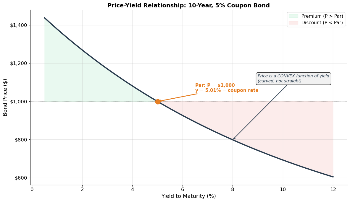
Key observations:
1. Price and yield move in OPPOSITE directions (inverse relationship)
2. The relationship is CONVEX (curved, not linear) — this matters for risk!
3. At par: price = $1,000 when yield = coupon rate (5%)
7. Bond Price Properties
The Inverse Relationship
When yields rise, bond prices fall — and vice versa. This is the fundamental source of interest rate risk for bond investors.
Sensitivity Depends on Maturity and Coupon
Longer maturity → more sensitive to yield changes (more cash flows far in the future, more heavily discounted).
Lower coupon → more sensitive to yield changes (more of the bond’s value comes from the distant principal payment).
A zero-coupon bond is the most sensitive for a given maturity.
Pull to Par
As a bond approaches maturity, its price converges to the face value — regardless of whether it was trading at a premium or discount. This is the pull-to-par effect.
Source
# ============================================================
# Sensitivity: Maturity and Coupon Effects
# ============================================================
yields = np.linspace(0.01, 0.10, 200)

fig, (ax1, ax2) = plt.subplots(1, 2, figsize=(14, 6))

# Left: Different maturities, same coupon
colors_m = ['#2ecc71', '#3498db', '#e67e22', '#e74c3c', '#8e44ad']
for T, color in zip([2, 5, 10, 20, 30], colors_m):
    prices = [bond_price_from_ytm(1000, 0.05, T, y) for y in yields]
    ax1.plot(yields * 100, prices, color=color, linewidth=2, label=f'T = {T} years')

ax1.axhline(y=1000, color='gray', linewidth=1, linestyle=':', alpha=0.5)
ax1.set_xlabel('Yield (%)', fontsize=12)
ax1.set_ylabel('Price ($)', fontsize=12)
ax1.set_title('Effect of Maturity\n(5% coupon, varying T)', fontsize=13, fontweight='bold')
ax1.legend(fontsize=10)
ax1.yaxis.set_major_formatter(mticker.FuncFormatter(lambda x, _: f'${x:,.0f}'))

# Right: Different coupons, same maturity
colors_c = ['#e74c3c', '#e67e22', '#3498db', '#2ecc71', '#8e44ad']
for c, color in zip([0.00, 0.02, 0.05, 0.08, 0.10], colors_c):
    prices = [bond_price_from_ytm(1000, c, 10, y) for y in yields]
    label = f'c = {c:.0%}' + (' (zero-coupon)' if c == 0 else '')
    ax2.plot(yields * 100, prices, color=color, linewidth=2, label=label)

ax2.axhline(y=1000, color='gray', linewidth=1, linestyle=':', alpha=0.5)
ax2.set_xlabel('Yield (%)', fontsize=12)
ax2.set_title('Effect of Coupon Rate\n(T = 10 years, varying c)', fontsize=13, fontweight='bold')
ax2.legend(fontsize=10)
ax2.yaxis.set_major_formatter(mticker.FuncFormatter(lambda x, _: f'${x:,.0f}'))

plt.tight_layout()
plt.show()

print("Key insights:")
print("• Longer maturity → steeper price-yield curve → MORE interest rate risk")
print("• Lower coupon → steeper price-yield curve → MORE interest rate risk")
print("• Zero-coupon bonds are the MOST sensitive (all value in the terminal payment)")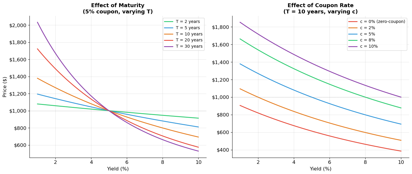
Key insights:
• Longer maturity → steeper price-yield curve → MORE interest rate risk
• Lower coupon → steeper price-yield curve → MORE interest rate risk
• Zero-coupon bonds are the MOST sensitive (all value in the terminal payment)
Source
# ============================================================
# Pull to Par — Bond Price Convergence Over Time
# ============================================================
# ▶ MODIFY AND RE-RUN
face = 1000
coupon_rate = 0.05
original_maturity = 20
market_yield = 0.07  # Bond bought when yields = 7% (discount bond)
# ============================================================

# Track price as remaining maturity shrinks
remaining = np.arange(original_maturity, 0, -0.25)
prices_discount = [bond_price_from_ytm(face, coupon_rate, T, market_yield) for T in remaining]

# Also a premium bond (yields = 3%)
prices_premium = [bond_price_from_ytm(face, coupon_rate, T, 0.03) for T in remaining]

# And a par bond
prices_par = [bond_price_from_ytm(face, coupon_rate, T, coupon_rate) for T in remaining]

fig, ax = plt.subplots(figsize=(12, 6))
time_elapsed = original_maturity - remaining

ax.plot(time_elapsed, prices_discount, color='#e74c3c', linewidth=2.5, label=f'Discount (y = {market_yield:.0%})')
ax.plot(time_elapsed, prices_premium, color='#2ecc71', linewidth=2.5, label='Premium (y = 3%)')
ax.plot(time_elapsed, prices_par, color='#3498db', linewidth=2, linestyle='--', label=f'Par (y = {coupon_rate:.0%})')
ax.axhline(y=face, color='#2c3e50', linewidth=1.5, linestyle=':', alpha=0.7)
ax.text(original_maturity * 0.95, face + 10, f'Par = ${face:,.0f}', fontsize=11, color='#2c3e50')

ax.set_xlabel('Years Elapsed', fontsize=12)
ax.set_ylabel('Bond Price ($)', fontsize=12)
ax.set_title(f'Pull to Par: {original_maturity}-Year, {coupon_rate:.0%} Coupon Bond\n(Assuming constant yields)',
             fontsize=14, fontweight='bold')
ax.yaxis.set_major_formatter(mticker.FuncFormatter(lambda x, _: f'${x:,.0f}'))
ax.legend(fontsize=11)
ax.annotate('All bonds converge\nto par at maturity', xy=(original_maturity - 1, face),
            xytext=(original_maturity - 5, face - 100), fontsize=11, style='italic',
            arrowprops=dict(arrowstyle='->', color='#2c3e50', lw=1.5))

plt.tight_layout()
plt.show()
---------------------------------------------------------------------------
TypeError Traceback (most recent call last)
Cell In[22], line 13
9 # ============================================================
10
11 # Track price as remaining maturity shrinks
12 remaining = np.arange(original_maturity, 0, -0.25)
---> 13 prices_discount = [bond_price_from_ytm(face, coupon_rate, T, market_yield) for T in remaining]
15 # Also a premium bond (yields = 3%)
16 prices_premium = [bond_price_from_ytm(face, coupon_rate, T, 0.03) for T in remaining]
Cell In[18], line 10, in bond_price_from_ytm(face, coupon_rate, maturity, ytm, freq)
8 n = maturity * freq
9 y = ytm / freq
---> 10 price = sum(C / (1 + y)**t for t in range(1, n + 1))
11 price += face / (1 + y)**n
12 return price
TypeError: 'numpy.float64' object cannot be interpreted as an integer8. Exercises
Exercise 1: STRIPS and Spot Rates
STRIPS are trading at the following prices (per $1 face):
| Maturity | 1 yr | 2 yr | 3 yr | 4 yr | 5 yr |
|---|---|---|---|---|---|
| Price | 0.9615 | 0.9151 | 0.8638 | 0.8096 | 0.7536 |
(a) Extract the spot rate for each maturity.
(b) Compute all one-year forward rates ().
(c) Verify that compounding forward rates recovers the spot rates.
(d) Is the term structure normal, inverted, or humped? What does the forward curve tell you about market expectations?
Source
# Exercise 1 — Workspace
# strip_prices = {1: 0.9615, 2: 0.9151, 3: 0.8638, 4: 0.8096, 5: 0.7536}
#
# (a) Spot rates
# for T, P in strip_prices.items():
#     r = (1/P)**(1/T) - 1
#     print(f"r(0,{T}) = {r:.4%}")
#
# (b) Forward rates
# spots = {T: (1/P)**(1/T) - 1 for T, P in strip_prices.items()}
# for T in range(2, 6):
#     f = (1 + spots[T])**T / (1 + spots[T-1])**(T-1) - 1
#     print(f"f_{T} = {f:.4%}")
Exercise 2: Coupon Bond Pricing
Using the STRIPS prices from Exercise 1:
(a) Price a 5-year, 6% annual coupon bond with $1,000 face value using spot rates.
(b) Compute the yield to maturity. How does it compare to the 5-year spot rate?
(c) Is this bond trading at a premium, discount, or par? Explain why.
(d) A trader observes this bond trading at $1,055 in the market. Is there an arbitrage? If so, describe the strategy and calculate the profit.
Source
# Exercise 2 — Workspace
# strip_prices = {1: 0.9615, 2: 0.9151, 3: 0.8638, 4: 0.8096, 5: 0.7536}
# spots = {T: (1/P)**(1/T) - 1 for T, P in strip_prices.items()}
#
# (a) Price with spot rates
# face, coupon_rate, T = 1000, 0.06, 5
# C = face * coupon_rate
# price = sum(C / (1 + spots[t])**t for t in range(1, T)) + (C + face) / (1 + spots[T])**T
# print(f"Bond price: ${price:,.2f}")
#
# (b) YTM
# ytm = compute_ytm(price, face, coupon_rate, T)
# print(f"YTM: {ytm:.4%} vs r(0,5) = {spots[5]:.4%}")
Exercise 3: Forward Rate Applications
(a) You observe 1-year and 2-year spot rates of 3% and 4% respectively. What is the implied forward rate ? If you believe the 1-year rate next year will be 4.5%, do you invest for 2 years at 4% or invest for 1 year at 3% and roll over? Explain.
(b) The following zero-coupon bond prices are observed:
| Maturity | 1 yr | 2 yr | 3 yr |
|---|---|---|---|
| Price | 0.9709 | 0.9335 | 0.8890 |
A client wants to borrow $5M in 2 years for 1 year. What rate should you quote? Describe the replicating strategy.
(c) If the expectations hypothesis holds (), what does an upward-sloping term structure imply about future short-term rates? If the liquidity preference hypothesis holds instead, what changes?
Source
# Exercise 3 — Workspace
# (a)
# r1, r2 = 0.03, 0.04
# f2 = (1 + r2)**2 / (1 + r1) - 1
# print(f"Implied forward rate f₂ = {f2:.4%}")
# # Compare: investing 2yr at 4% vs 1yr at 3% then 1yr at 4.5%
# return_2yr = (1 + r2)**2
# return_roll = (1 + r1) * (1 + 0.045)
# print(f"2-year strategy: {return_2yr:.6f}")
# print(f"Roll-over strategy: {return_roll:.6f}")
# print(f"Better strategy: {'Roll-over' if return_roll > return_2yr else '2-year lock-in'}")
#
# (b)
# prices_ex = {1: 0.9709, 2: 0.9335, 3: 0.8890}
# spots_ex = {T: (1/P)**(1/T) - 1 for T, P in prices_ex.items()}
# f3 = (1 + spots_ex[3])**3 / (1 + spots_ex[2])**2 - 1
# print(f"Quote for 1-year loan starting in 2 years: {f3:.4%}")
Key Takeaways — Session 4
Fixed-income securities are the largest asset class globally. Their cash flows are contractually fixed (in nominal terms), making valuation a direct NPV application.
Discount bonds (STRIPS) are the building blocks. Their prices directly reveal spot rates — the market’s required return for each maturity.
The term structure (spot rates plotted against maturity) contains rich information about market expectations and risk preferences.
Forward rates are extracted from the term structure via no-arbitrage. They represent the rate for a future loan implied by current prices — not a forecast, but an arbitrage-free pricing tool.
Coupon bonds = portfolios of discount bonds. This allows pricing via replication and is the basis for fixed-income arbitrage.
Yield to maturity is a convenient summary measure — the single rate that prices all cash flows — but it is a complex average of spot rates, not the “true” discount rate for any particular cash flow.
Bond prices are convex in yield: the price-yield relationship curves, not lines. Longer maturity and lower coupon → greater sensitivity to yield changes.
References
Brealey, R.A., Myers, S.C., and Allen, F. Principles of Corporate Finance, Chapters 23–25.
MIT OCW 15.401: Fixed-Income Securities
Sundaresan, S. (1997). Fixed Income Markets and Their Derivatives. South-Western.
Tuckman, B. (1995). Fixed Income Securities: Tools for Today’s Markets. Wiley.
Next: Session 5 — Fixed-Income Securities II — Duration, convexity, immunization, corporate bonds, credit risk, and the sub-prime crisis securitization example.