Lecture 6: Equities — Stock Valuation, the Dividend Discount Model, and Growth Opportunities
MIT 15.401 — Finance Theory I (Prof. Andrew Lo)
Video: MIT OCW — Equities
Readings: Brealey, Myers, and Allen — Chapter 4
This session transitions from fixed-income securities (known promised cash flows) to equities (uncertain cash flows). This is a major conceptual leap: unlike bonds, equity cash flows are not contractually fixed — dividends are uncertain in both magnitude and timing, and the terminal price is unknown. Yet the fundamental valuation framework remains the same: price = present value of expected future cash flows.
The workhorse model is the Dividend Discount Model (DDM), which values a stock as the present value of all future dividends. When we add a constant growth assumption, this becomes the Gordon Growth Model — one of the most famous formulas in finance: .
We then connect dividends to earnings through the payout ratio, define growth opportunities, and show how the P/E ratio decomposes into a no-growth component and the present value of growth opportunities (PVGO).
Table of Contents
Source
# ============================================================
# Setup
# ============================================================
import numpy as np
import pandas as pd
import matplotlib.pyplot as plt
import matplotlib.ticker as mticker
from scipy.optimize import brentq

plt.rcParams.update({
    'figure.figsize': (10, 5),
    'axes.spines.top': False,
    'axes.spines.right': False,
    'axes.grid': True,
    'grid.alpha': 0.3,
    'font.size': 12,
    'lines.linewidth': 2,
})

print("Libraries loaded successfully.")
Libraries loaded successfully.
1. Industry Overview — The Equity Market
What Is Common Stock?
Common stock represents an ownership position (equity) in a corporation. Key characteristics:
Residual claimant: stockholders get paid after all other obligations (bondholders, employees, taxes). This makes equity riskier than debt — but also gives unlimited upside.
Limited liability: shareholders can lose at most their investment. They are not personally liable for corporate debts.
Voting rights: shareholders elect the board of directors.
Dividends: payouts in cash or stock, at the discretion of the board. Unlike bond coupons, dividends are not contractually guaranteed.
Access to public markets: shares can be bought and sold on exchanges.
Equity vs. Bonds — The Fundamental Distinction
| Feature | Bonds | Equities |
|---|---|---|
| Cash flows | Contractually fixed | Uncertain |
| Priority | Senior claim | Residual claim |
| Upside | Capped at face value | Unlimited |
| Downside | Loss if default | Can go to zero |
| Tax treatment | Interest is deductible | Dividends paid from after-tax income |
| Maturity | Finite | Perpetual |
Markets
Primary market: IPOs, SEOs, venture capital — companies raise capital by issuing new shares. Secondary market: NYSE, NASDAQ, AMEX — investors trade existing shares among themselves. The secondary market provides liquidity and price discovery.
Source
# ============================================================
# Equity Market Scale — IPOs and Market Activity
# ============================================================
# Lo's slide data: IPO volume and total underwriting 1990-2004
years = list(range(1990, 2005))
ipo_volume = [5, 16, 24, 41, 28, 30, 50, 43, 37, 64, 76, 36, 26, 16, 48]  # $B
total_underwriting = [312, 587, 856, 1063, 716, 722, 979, 1317, 1868, 1960, 1851, 2535, 2581, 2890, 2859]

fig, (ax1, ax2) = plt.subplots(1, 2, figsize=(14, 6))

# IPOs
colors_ipo = ['#e74c3c' if v > 60 else '#3498db' for v in ipo_volume]
ax1.bar(years, ipo_volume, color=colors_ipo, alpha=0.8, edgecolor='white')
ax1.set_xlabel('Year', fontsize=12)
ax1.set_ylabel('IPO Volume ($B)', fontsize=12)
ax1.set_title('Initial Public Offerings\n(US Market)', fontsize=14, fontweight='bold')
ax1.tick_params(axis='x', rotation=45)

# Highlight dot-com boom
ax1.annotate('Dot-com\nboom', xy=(2000, 76), xytext=(1997, 80),
            fontsize=10, color='#e74c3c', fontweight='bold',
            arrowprops=dict(arrowstyle='->', color='#e74c3c'))

# Total underwriting
ax2.bar(years, [v/1000 for v in total_underwriting], color='#2c3e50', alpha=0.8, edgecolor='white')
ax2.set_xlabel('Year', fontsize=12)
ax2.set_ylabel('Total Underwriting ($T)', fontsize=12)
ax2.set_title('Total Securities Underwriting\n(US Market)', fontsize=14, fontweight='bold')
ax2.tick_params(axis='x', rotation=45)

plt.tight_layout()
plt.show()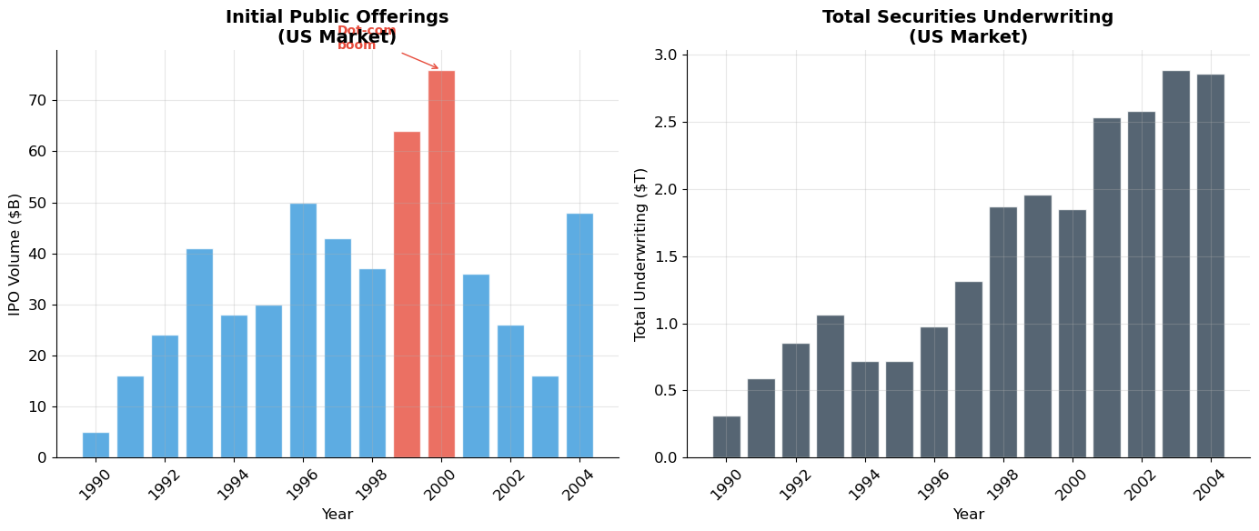
2. The Dividend Discount Model (DDM)
The Core Idea
How should we value a stock? The same way we value any asset: as the present value of its future cash flows. For a stock, the relevant cash flows are dividends.
One-Period Model
If you hold a stock for one period, you receive a dividend and sell at price :
But what determines ? The next investor’s expected dividend and resale price:
Multi-Period Model
Substituting recursively and pushing the terminal price to infinity:
This is the Dividend Discount Model: the stock price equals the present value of all future dividends, to infinity.
Key Assumptions (for the basic version)
Constant discount rate across all periods
Dividends are the only relevant cash flows to equity holders
The terminal price grows slower than the discount rate (ensuring convergence)
Critical insight: Even though any individual investor may hold the stock for a short period and sell it, the price today still equals the PV of all future dividends — because the price the next investor pays is itself based on future dividends.
Source
# ============================================================
# One-Period vs. Multi-Period DDM — Equivalence Demonstration
# ============================================================

def ddm_general(dividends, terminal_price, r):
    """Value a stock from a finite list of dividends plus terminal price."""
    T = len(dividends)
    pv = sum(D / (1 + r)**t for t, D in enumerate(dividends, 1))
    pv += terminal_price / (1 + r)**T
    return pv


# Example: constant dividend stream, showing equivalence
r = 0.12
D = 2.00  # constant dividend forever

# Investor 1: holds for 1 year
# P1 = D/r (perpetuity from year 2 onward)
P1 = D / r
P0_1period = ddm_general([D], P1, r)

# Investor 2: holds for 5 years
P5 = D / r  # same perpetuity from year 6
P0_5period = ddm_general([D]*5, P5, r)

# Investor 3: holds forever (perpetuity formula)
P0_forever = D / r

print("=" * 60)
print("DDM EQUIVALENCE: Holding Period Doesn't Matter")
print(f"Constant dividend D = ${D:.2f}, discount rate r = {r:.0%}")
print("=" * 60)
print(f"1-year holding period:  P₀ = (D₁ + P₁)/(1+r) = ({D} + {P1:.2f})/1.12 = ${P0_1period:.4f}")
print(f"5-year holding period:  P₀ = Σ PV(D) + PV(P₅)                       = ${P0_5period:.4f}")
print(f"Infinite holding:       P₀ = D/r = {D}/{r}                            = ${P0_forever:.4f}")
print(f"\n→ All methods give P₀ = ${D/r:.2f} regardless of holding period ✓")
print(f"  The stock price today reflects ALL future dividends, not just")
print(f"  the dividends you personally will receive while holding it.")
============================================================
DDM EQUIVALENCE: Holding Period Doesn't Matter
Constant dividend D = $2.00, discount rate r = 12%
============================================================
1-year holding period: P₀ = (D₁ + P₁)/(1+r) = (2.0 + 16.67)/1.12 = $16.6667
5-year holding period: P₀ = Σ PV(D) + PV(P₅) = $16.6667
Infinite holding: P₀ = D/r = 2.0/0.12 = $16.6667
→ All methods give P₀ = $16.67 regardless of holding period ✓
The stock price today reflects ALL future dividends, not just
the dividends you personally will receive while holding it.
Source
# ============================================================
# DDM Convergence: How Much Value Comes From Near vs. Far Dividends?
# ============================================================
# ▶ MODIFY AND RE-RUN
D = 2.00
r = 0.10
g = 0.04  # growth rate
# ============================================================

# Gordon Growth Model value
P0 = D * (1 + g) / (r - g)

# Cumulative PV of dividends from year 1 to T
T_max = 100
cumulative_pv = np.zeros(T_max)
for t in range(1, T_max + 1):
    Dt = D * (1 + g)**t
    cumulative_pv[t-1] = cumulative_pv[t-2] + Dt / (1 + r)**t if t > 1 else Dt / (1 + r)

fig, (ax1, ax2) = plt.subplots(1, 2, figsize=(14, 6))

# Left: Individual PV contributions
T_show = 50
pvs = [D * (1 + g)**t / (1 + r)**t for t in range(1, T_show + 1)]
ax1.bar(range(1, T_show + 1), pvs, color='#3498db', alpha=0.7, width=0.8)
ax1.set_xlabel('Year', fontsize=12)
ax1.set_ylabel('PV of Dividend ($)', fontsize=12)
ax1.set_title(f'PV of Each Year\'s Dividend\n(D₀=${D}, g={g:.0%}, r={r:.0%})', fontsize=13, fontweight='bold')

# Right: Cumulative
years = np.arange(1, T_max + 1)
ax2.plot(years, cumulative_pv, color='#2c3e50', linewidth=3)
ax2.axhline(y=P0, color='#e74c3c', linewidth=2, linestyle='--', label=f'Gordon Model: P₀ = ${P0:.2f}')

# Milestones
for pct in [0.5, 0.75, 0.9]:
    idx = np.searchsorted(cumulative_pv, P0 * pct)
    if idx < T_max:
        ax2.plot(idx + 1, cumulative_pv[idx], 'o', color='#e67e22', markersize=8, zorder=5)
        ax2.annotate(f'{pct:.0%} in ~{idx+1} years', xy=(idx + 1, cumulative_pv[idx]),
                    xytext=(idx + 10, cumulative_pv[idx] - P0 * 0.05), fontsize=9,
                    arrowprops=dict(arrowstyle='->', color='#e67e22'))

ax2.set_xlabel('Years of Dividends Included', fontsize=12)
ax2.set_ylabel('Cumulative PV ($)', fontsize=12)
ax2.set_title('Convergence to Full DDM Value', fontsize=13, fontweight='bold')
ax2.legend(fontsize=11)

plt.tight_layout()
plt.show()

for pct in [0.5, 0.75, 0.9, 0.95]:
    idx = np.searchsorted(cumulative_pv, P0 * pct) + 1
    print(f"  {pct:.0%} of value captured in first {idx:>3d} years")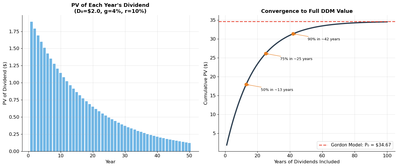
  50% of value captured in first  13 years
  75% of value captured in first  25 years
  90% of value captured in first  42 years
  95% of value captured in first  54 years
3. The Gordon Growth Model
Derivation
If dividends grow at a constant rate forever, with :
The DDM becomes a growing perpetuity (which we derived in Session 2):
This is the Gordon Growth Model (Gordon, 1959) — perhaps the single most important formula in equity valuation.
Lo’s Example (Slide 10)
Dividends grow at per year, current dividend , expected return :
The Three Determinants of Stock Price
The Gordon model reveals that stock price depends on exactly three things:
(expected next dividend): higher dividends → higher price
(required return / cost of equity): higher risk → lower price
(dividend growth rate): higher growth → higher price
And the model gives a precise formula for how sensitive the price is to each.
Source
# ============================================================
# Gordon Growth Model — Core Calculations
# ============================================================

def gordon_growth_price(D0, r, g):
    """Gordon Growth Model: P0 = D0*(1+g)/(r-g). Requires r > g."""
    if r <= g:
        return float('inf')
    return D0 * (1 + g) / (r - g)


# Lo's example
D0 = 1.00
r = 0.20
g = 0.06
P0 = gordon_growth_price(D0, r, g)

print("=" * 60)
print("GORDON GROWTH MODEL — Lo's Example")
print("=" * 60)
print(f"Current dividend D₀ = ${D0:.2f}")
print(f"Growth rate g = {g:.0%}")
print(f"Required return r = {r:.0%}")
print(f"\nP₀ = D₀(1+g)/(r-g) = ${D0}×{1+g:.2f}/({r:.2f}-{g:.2f}) = ${P0:.2f}")

# Sensitivity table
print(f"\n{'':>8s}", end='')
for g_val in [0.02, 0.04, 0.06, 0.08, 0.10, 0.12]:
    print(f"{'g='+f'{g_val:.0%}':>9s}", end='')
print()
print("-" * 62)

for r_val in [0.12, 0.14, 0.16, 0.18, 0.20, 0.25]:
    print(f"r={r_val:.0%}  ", end='')
    for g_val in [0.02, 0.04, 0.06, 0.08, 0.10, 0.12]:
        if r_val > g_val:
            p = gordon_growth_price(1.0, r_val, g_val)
            print(f" ${p:>6.2f}", end='')
        else:
            print(f"     ∞ ", end='')
    print()

print("\nKey insight: Price is EXTREMELY sensitive to (r-g).")
print("A small change in growth or discount rate has a massive impact on valuation.")
============================================================
GORDON GROWTH MODEL — Lo's Example
============================================================
Current dividend D₀ = $1.00
Growth rate g = 6%
Required return r = 20%
P₀ = D₀(1+g)/(r-g) = $1.0×1.06/(0.20-0.06) = $7.57
g=2% g=4% g=6% g=8% g=10% g=12%
--------------------------------------------------------------
r=12% $ 10.20 $ 13.00 $ 17.67 $ 27.00 $ 55.00 ∞
r=14% $ 8.50 $ 10.40 $ 13.25 $ 18.00 $ 27.50 $ 56.00
r=16% $ 7.29 $ 8.67 $ 10.60 $ 13.50 $ 18.33 $ 28.00
r=18% $ 6.38 $ 7.43 $ 8.83 $ 10.80 $ 13.75 $ 18.67
r=20% $ 5.67 $ 6.50 $ 7.57 $ 9.00 $ 11.00 $ 14.00
r=25% $ 4.43 $ 4.95 $ 5.58 $ 6.35 $ 7.33 $ 8.62
Key insight: Price is EXTREMELY sensitive to (r-g).
A small change in growth or discount rate has a massive impact on valuation.
Source
# ============================================================
# Sensitivity Analysis: Price vs. Growth Rate and Discount Rate
# ============================================================
fig, (ax1, ax2) = plt.subplots(1, 2, figsize=(14, 6))

# Left: Price vs. growth rate (fixed r)
g_range = np.linspace(0, 0.095, 200)
for r_val, color, ls in [(0.10, '#e74c3c', '-'), (0.12, '#e67e22', '--'),
                          (0.15, '#3498db', '-'), (0.20, '#2c3e50', '--')]:
    prices = [gordon_growth_price(1.0, r_val, g) for g in g_range]
    ax1.plot(g_range * 100, prices, color=color, linewidth=2, linestyle=ls,
            label=f'r = {r_val:.0%}')

ax1.set_xlabel('Growth Rate g (%)', fontsize=12)
ax1.set_ylabel('Stock Price ($)', fontsize=12)
ax1.set_title('Price vs. Growth Rate\n(D₀ = $1.00)', fontsize=14, fontweight='bold')
ax1.set_ylim(0, 60)
ax1.legend(fontsize=10)
ax1.annotate('Price explodes\nas g → r', xy=(8.5, 50), fontsize=10, color='#e74c3c',
            style='italic', bbox=dict(boxstyle='round', facecolor='#fdf2f2', alpha=0.9))

# Right: Price vs. discount rate (fixed g)
r_range = np.linspace(0.05, 0.25, 200)
for g_val, color, ls in [(0.02, '#2ecc71', '-'), (0.04, '#3498db', '--'),
                          (0.06, '#e67e22', '-'), (0.08, '#e74c3c', '--')]:
    prices = [gordon_growth_price(1.0, r, g_val) if r > g_val else np.nan for r in r_range]
    ax2.plot(r_range * 100, prices, color=color, linewidth=2, linestyle=ls,
            label=f'g = {g_val:.0%}')

ax2.set_xlabel('Required Return r (%)', fontsize=12)
ax2.set_ylabel('Stock Price ($)', fontsize=12)
ax2.set_title('Price vs. Discount Rate\n(D₀ = $1.00)', fontsize=14, fontweight='bold')
ax2.set_ylim(0, 60)
ax2.legend(fontsize=10)

plt.tight_layout()
plt.show()

print("The Gordon model has a singularity at g = r (price → ∞).")
print("In practice, g must be STRICTLY less than r for the model to be valid.")
print("For mature companies, g should not exceed nominal GDP growth (roughly 4-6%).")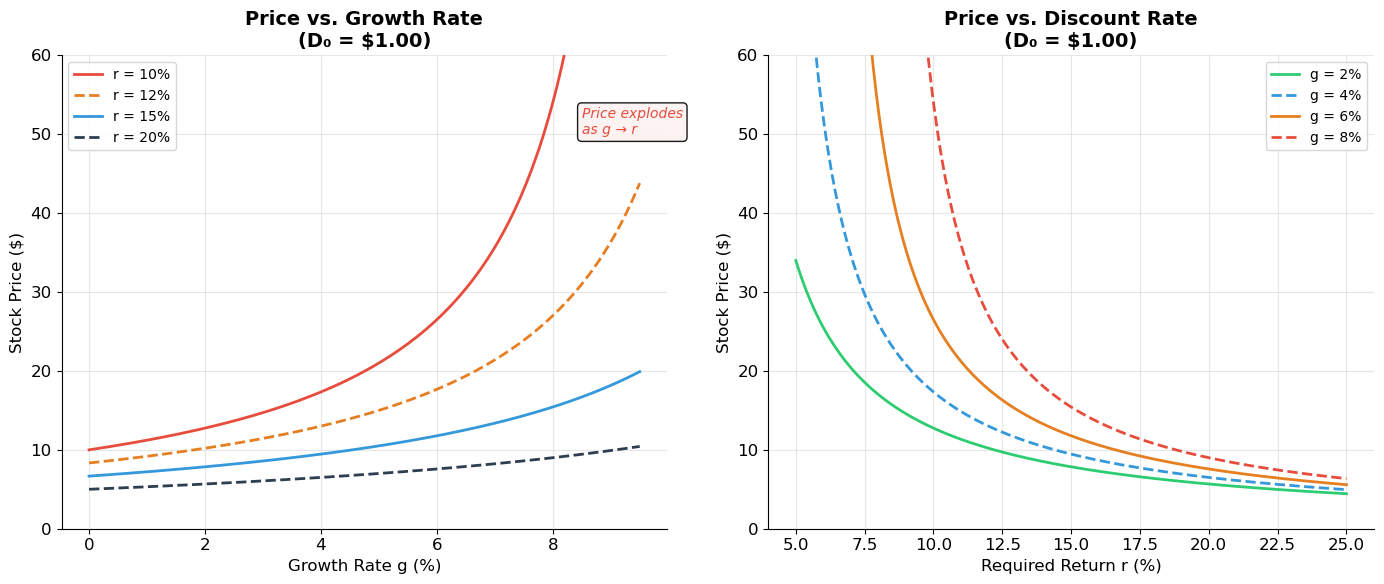
The Gordon model has a singularity at g = r (price → ∞).
In practice, g must be STRICTLY less than r for the model to be valid.
For mature companies, g should not exceed nominal GDP growth (roughly 4-6%).
4. Estimating the Cost of Equity from the DDM
Rearranging the Gordon Model
The Gordon model can be solved for the discount rate (cost of equity):
This decomposition is intuitive: the return to an equity investor comes from two sources:
Dividend yield (): income from dividends
Capital gains (): price appreciation
Lo’s Duke Power Example (Slide 11)
In September 1992, Duke Power had:
Dividend yield:
Growth estimates: Value Line (5.0%), IBES (5.5%), historical (4.1%)
Using different growth estimates:
| Source | ≈ | ||
|---|---|---|---|
| Value Line | 5.0% | ~5.5% | ~10.5% |
| IBES | 5.5% | ~5.5% | ~11.0% |
| Historical | 4.1% | ~5.4% | ~9.5% |
The cost of equity for a utility like Duke Power: roughly 10–11%.
Source
# ============================================================
# Cost of Equity Estimation — Duke Power Example
# ============================================================
D0_P0 = 0.052  # current dividend yield

growth_estimates = {
    'Value Line': 0.050,
    'IBES Consensus': 0.055,
    'Historical': 0.041,
}

print("=" * 60)
print("COST OF EQUITY — Duke Power (September 1992)")
print("=" * 60)
print(f"Current dividend yield D₀/P₀ = {D0_P0:.1%}")
print()
print(f"{'Source':>18s} {'g':>8s} {'D₁/P₀':>10s} {'r = D₁/P₀ + g':>15s}")
print("-" * 55)

r_estimates = []
for source, g in growth_estimates.items():
    D1_P0 = D0_P0 * (1 + g)
    r = D1_P0 + g
    r_estimates.append(r)
    print(f"{source:>18s} {g:>8.1%} {D1_P0:>10.2%} {r:>15.2%}")

print(f"\nRange of cost of equity estimates: {min(r_estimates):.1%} to {max(r_estimates):.1%}")
print(f"Average: {np.mean(r_estimates):.1%}")
print("\nNote: Duke Power is a regulated utility — low risk, stable dividends.")
print("Its cost of equity is correspondingly modest (~10%) compared to")
print("high-growth tech firms (which might have r = 15-20%).")
============================================================
COST OF EQUITY — Duke Power (September 1992)
============================================================
Current dividend yield D₀/P₀ = 5.2%
Source g D₁/P₀ r = D₁/P₀ + g
-------------------------------------------------------
Value Line 5.0% 5.46% 10.46%
IBES Consensus 5.5% 5.49% 10.99%
Historical 4.1% 5.41% 9.51%
Range of cost of equity estimates: 9.5% to 11.0%
Average: 10.3%
Note: Duke Power is a regulated utility — low risk, stable dividends.
Its cost of equity is correspondingly modest (~10%) compared to
high-growth tech firms (which might have r = 15-20%).
Source
# ============================================================
# Return Decomposition: Dividend Yield vs. Capital Gains
# ============================================================
# Show how return composition changes with growth rate

g_range = np.linspace(0, 0.09, 200)
r_fixed = 0.12
D0 = 1.0

div_yields = np.array([D0 * (1 + g) / gordon_growth_price(D0, r_fixed, g) if r_fixed > g else np.nan for g in g_range])
cap_gains = g_range

fig, ax = plt.subplots(figsize=(11, 6))

ax.fill_between(g_range * 100, 0, div_yields * 100, alpha=0.4, color='#3498db', label='Dividend Yield')
ax.fill_between(g_range * 100, div_yields * 100, (div_yields + cap_gains) * 100,
                alpha=0.4, color='#e67e22', label='Capital Gains (g)')

ax.axhline(y=r_fixed * 100, color='#2c3e50', linewidth=2, linestyle='--', label=f'Total Return = r = {r_fixed:.0%}')

ax.set_xlabel('Growth Rate g (%)', fontsize=13)
ax.set_ylabel('Return Component (%)', fontsize=13)
ax.set_title('Return Decomposition: r = Dividend Yield + Capital Gains',
             fontsize=14, fontweight='bold')
ax.legend(fontsize=11)
ax.set_ylim(0, 14)
ax.set_xlim(0, 9)

# Annotations
ax.annotate('Low-growth (utilities):\nhigh dividend yield', xy=(1.5, 10), fontsize=10,
            color='#3498db', fontweight='bold',
            bbox=dict(boxstyle='round', facecolor='#eaf2f8', alpha=0.9))
ax.annotate('High-growth (tech):\nlow dividend yield,\nhigh capital gains', xy=(6.5, 5), fontsize=10,
            color='#e67e22', fontweight='bold',
            bbox=dict(boxstyle='round', facecolor='#fdf6e3', alpha=0.9))

plt.tight_layout()
plt.show()

print("The total return is always r (by the Gordon model: r = D₁/P₀ + g).")
print("As growth increases, the mix shifts from dividend yield to capital gains.")
print("This is why growth stocks have low dividend yields — it's not a flaw!")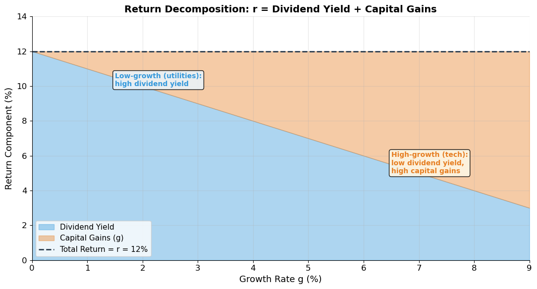
The total return is always r (by the Gordon model: r = D₁/P₀ + g).
As growth increases, the mix shifts from dividend yield to capital gains.
This is why growth stocks have low dividend yields — it's not a flaw!
5. Multi-Stage Growth Models
Why Multi-Stage?
The constant-growth assumption is unrealistic for many companies. Firms typically pass through distinct phases:
Growth stage: rapid expansion, high profit margins, heavy reinvestment, low dividend payout
Transition stage: competition erodes margins, growth slows, investment opportunities decline
Mature stage: stable growth, high payout ratio, earnings grow at or below GDP rate
Two-Stage DDM
The most common variant assumes high growth for years, then stable growth forever:
where the terminal value uses the Gordon model:
Lo’s Example (Slide 12)
A company with , grows at for 7 years, then thereafter.
Source
# ============================================================
# Two-Stage Growth DDM
# ============================================================

def two_stage_ddm(D0, r, g_high, T_high, g_low):
    """Two-stage DDM: high growth for T years, then stable growth forever."""
    # Phase 1: high-growth dividends
    phase1_pv = 0
    DT = D0
    for t in range(1, T_high + 1):
        DT = D0 * (1 + g_high)**t
        phase1_pv += DT / (1 + r)**t

    # Phase 2: terminal value using Gordon model
    D_terminal = DT * (1 + g_low)
    P_T = D_terminal / (r - g_low) if r > g_low else float('inf')
    phase2_pv = P_T / (1 + r)**T_high

    return phase1_pv, phase2_pv, phase1_pv + phase2_pv


# Lo's example
D0 = 1.00
r = 0.20
g_H = 0.06
T = 7
g_L = 0.00

pv1, pv2, P0 = two_stage_ddm(D0, r, g_H, T, g_L)

print("=" * 60)
print("TWO-STAGE DDM — Lo's Example")
print("=" * 60)
print(f"D₀ = ${D0:.2f}, r = {r:.0%}, g_H = {g_H:.0%} (years 1–{T}), g_L = {g_L:.0%} (year {T+1}+)")
print()

# Show dividend timeline
print("Dividend timeline:")
for t in range(1, T + 2):
    Dt = D0 * (1 + g_H)**min(t, T)
    if t > T:
        Dt = D0 * (1 + g_H)**T * (1 + g_L)
    phase = "← high growth" if t <= T else "← stable"
    print(f"  D_{t} = ${Dt:.4f}  {phase}")
    if t == T + 1:
        break

# Terminal price
D_T = D0 * (1 + g_H)**T
P_T = D_T * (1 + g_L) / (r - g_L)

print(f"\nTerminal value at T={T}: P_{T} = D_{T+1}/(r-g_L) = ${D_T*(1+g_L):.4f}/{r-g_L:.2f} = ${P_T:.2f}")
print(f"\nPV of high-growth dividends (years 1–{T}): ${pv1:.4f}")
print(f"PV of terminal value:                      ${pv2:.4f}")
print(f"Total stock price P₀:                      ${P0:.4f}")
print(f"\nTerminal value share: {pv2/(pv1+pv2)*100:.1f}% of total value")

# Compare with pure Gordon models
P0_allhigh = gordon_growth_price(D0, r, g_H)
P0_no_growth = D0 * (1 + 0) / (r - 0)  # g=0 forever

print(f"\nComparison:")
print(f"  If g = {g_H:.0%} forever:   P₀ = ${P0_allhigh:.2f}")
print(f"  Two-stage model:     P₀ = ${P0:.2f}")
print(f"  If g = {g_L:.0%} forever:   P₀ = ${P0_no_growth:.2f}")
============================================================
TWO-STAGE DDM — Lo's Example
============================================================
D₀ = $1.00, r = 20%, g_H = 6% (years 1–7), g_L = 0% (year 8+)
Dividend timeline:
D_1 = $1.0600 ← high growth
D_2 = $1.1236 ← high growth
D_3 = $1.1910 ← high growth
D_4 = $1.2625 ← high growth
D_5 = $1.3382 ← high growth
D_6 = $1.4185 ← high growth
D_7 = $1.5036 ← high growth
D_8 = $1.5036 ← stable
Terminal value at T=7: P_7 = D_8/(r-g_L) = $1.5036/0.20 = $7.52
PV of high-growth dividends (years 1–7): $4.3942
PV of terminal value: $2.0982
Total stock price P₀: $6.4924
Terminal value share: 32.3% of total value
Comparison:
If g = 6% forever: P₀ = $7.57
Two-stage model: P₀ = $6.49
If g = 0% forever: P₀ = $5.00
Source
# ============================================================
# Visualization: Two-Stage DDM Cash Flows and Valuation
# ============================================================
# ▶ MODIFY AND RE-RUN
D0 = 2.00
r = 0.12
g_high = 0.15     # high-growth phase
T_high = 5        # years of high growth
g_low = 0.04      # stable growth
# ============================================================

pv1, pv2, P0 = two_stage_ddm(D0, r, g_high, T_high, g_low)

# Build dividend series
T_plot = 25
divs = []
pvs = []
for t in range(1, T_plot + 1):
    if t <= T_high:
        Dt = D0 * (1 + g_high)**t
    else:
        Dt = D0 * (1 + g_high)**T_high * (1 + g_low)**(t - T_high)
    divs.append(Dt)
    pvs.append(Dt / (1 + r)**t)

fig, (ax1, ax2) = plt.subplots(1, 2, figsize=(14, 6))

# Left: Dividend timeline
years_plot = range(1, T_plot + 1)
colors_bar = ['#e74c3c' if t <= T_high else '#3498db' for t in years_plot]
ax1.bar(years_plot, divs, color=colors_bar, alpha=0.75, edgecolor='white')
ax1.axvline(x=T_high + 0.5, color='#2c3e50', linewidth=2, linestyle=':', alpha=0.7)
ax1.text(T_high / 2, max(divs) * 0.9, f'High Growth\n(g = {g_high:.0%})',
         ha='center', fontsize=11, color='#e74c3c', fontweight='bold')
ax1.text(T_high + (T_plot - T_high) / 2, max(divs) * 0.9, f'Stable Growth\n(g = {g_low:.0%})',
         ha='center', fontsize=11, color='#3498db', fontweight='bold')
ax1.set_xlabel('Year', fontsize=12)
ax1.set_ylabel('Dividend ($)', fontsize=12)
ax1.set_title('Expected Dividend Stream', fontsize=14, fontweight='bold')

# Right: PV contributions
ax2.bar(years_plot, pvs, color=colors_bar, alpha=0.75, edgecolor='white')
ax2.axvline(x=T_high + 0.5, color='#2c3e50', linewidth=2, linestyle=':', alpha=0.7)

# Show cumulative reaching total
cumulative = np.cumsum(pvs)
ax2_twin = ax2.twinx()
ax2_twin.plot(years_plot, cumulative, color='#2c3e50', linewidth=2.5, marker='o', markersize=3)
ax2_twin.axhline(y=P0, color='#e67e22', linewidth=2, linestyle='--')
ax2_twin.set_ylabel('Cumulative PV ($)', fontsize=12, color='#2c3e50')
ax2_twin.tick_params(axis='y', colors='#2c3e50')

ax2.set_xlabel('Year', fontsize=12)
ax2.set_ylabel('PV of Dividend ($)', fontsize=12)
ax2.set_title(f'PV of Each Dividend (P₀ = ${P0:.2f})', fontsize=14, fontweight='bold')

plt.tight_layout()
plt.show()

print(f"Two-stage DDM: P₀ = ${P0:.2f}")
print(f"  PV of high-growth dividends: ${pv1:.2f} ({pv1/P0*100:.1f}%)")
print(f"  PV of terminal value:        ${pv2:.2f} ({pv2/P0*100:.1f}%)")
print(f"\nThe terminal value typically dominates — most of a stock's value")
print(f"comes from the LONG-RUN growth phase, not the near-term high growth.")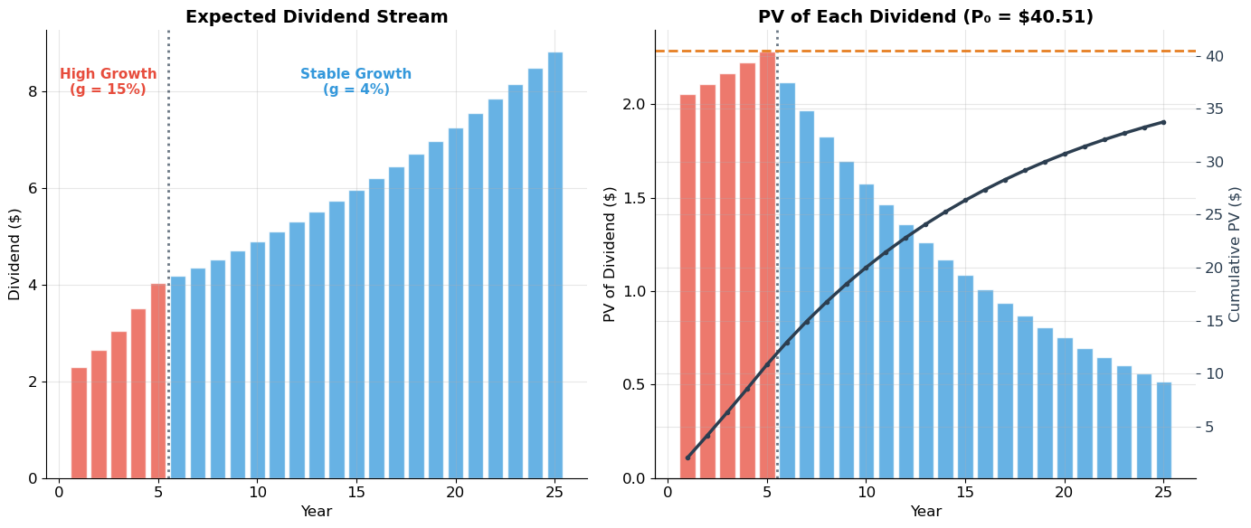
Two-stage DDM: P₀ = $40.51
  PV of high-growth dividends: $10.83 (26.7%)
  PV of terminal value:        $29.67 (73.3%)

The terminal value typically dominates — most of a stock's value
comes from the LONG-RUN growth phase, not the near-term high growth.
6. EPS, P/E, and the Link to Earnings
From Dividends to Earnings
In practice, forecasting individual dividends is difficult. Analysts often work with earnings and payout ratios instead.
Key Definitions
| Concept | Symbol | Definition |
|---|---|---|
| Earnings per share | EPS | Net income / shares outstanding |
| Payout ratio | DPS / EPS (fraction of earnings paid as dividends) | |
| Plowback (retention) ratio | 1 − (fraction reinvested) | |
| Book value per share | BV | Cumulative retained earnings per share |
| Return on book equity | ROE | EPS / BV |
The Sustainable Growth Rate
If a company reinvests fraction of earnings at return ROE:
This is the sustainable growth rate — the rate at which earnings (and dividends) can grow without external financing.
Lo’s Texas Western Example (Slides 14–16)
Texas Western (TW) has:
Expected EPS₁ = $1.00, Book Value = $10.00
Plans to grow net book assets by 8% per year (financed by retained earnings)
Discount rate = 10% = ROE
Key ratios:
Plowback ratio:
Payout ratio:
ROE = EPS / BV = 1/10 = 10%
Sustainable growth: ✓
Source
# ============================================================
# Texas Western Example — EPS, Growth, and Valuation
# ============================================================

# Company parameters
EPS1 = 1.00
BV0 = 10.00
g = 0.08
r = 0.10
ROE = EPS1 / BV0  # = 10%
b = BV0 * g / EPS1  # plowback ratio
p = 1 - b             # payout ratio
D1 = EPS1 * p         # dividend per share

print("=" * 60)
print("TEXAS WESTERN — Lo's Example")
print("=" * 60)
print(f"EPS₁ = ${EPS1:.2f},  BV₀ = ${BV0:.2f}")
print(f"ROE = EPS/BV = {ROE:.0%}")
print(f"Growth rate g = {g:.0%}")
print(f"Plowback ratio b = {b:.2f}")
print(f"Payout ratio p = {p:.2f}")
print(f"DPS₁ = EPS × p = ${D1:.2f}")
print(f"Sustainable growth: b × ROE = {b:.2f} × {ROE:.2f} = {b * ROE:.0%} = g ✓")

# CASE 1: Expand at 8% forever
P0_case1 = D1 / (r - g)
print(f"\nCase 1: Expand at {g:.0%} forever")
print(f"  P₀ = D₁/(r-g) = {D1}/{r}-{g} = ${P0_case1:.2f}")
print(f"  P/E = {P0_case1/EPS1:.1f}×")

# CASE 2: Growth slows to 4% after year 5
g_high = 0.08
g_low = 0.04
T_trans = 5

# Build explicit year-by-year forecast
print(f"\nCase 2: {g_high:.0%} for {T_trans} years, then {g_low:.0%}")
print(f"\n{'Year':>6s} {'BV_start':>10s} {'EPS':>8s} {'Inv':>8s} {'DPS':>8s} {'b':>6s}")
print("-" * 55)

# Phase 1
BV_t = BV0
EPS_t = EPS1
pv_divs = 0
for t in range(1, T_trans + 1):
    EPS_t = BV_t * ROE
    inv_t = BV_t * g_high
    D_t = EPS_t - inv_t
    pv_divs += D_t / (1 + r)**t
    b_t = inv_t / EPS_t
    print(f"{t:>6d} {BV_t:>10.4f} {EPS_t:>8.4f} {inv_t:>8.4f} {D_t:>8.4f} {b_t:>6.2f}")
    BV_t = BV_t * (1 + g_high)

# Terminal value: from year T+1, ROE still 10% but growth drops to 4%
# New plowback: b_new = g_low / ROE
b_new = g_low / ROE
p_new = 1 - b_new
EPS_T1 = BV_t * ROE
D_T1 = EPS_T1 * p_new
P_T = D_T1 / (r - g_low)
pv_terminal = P_T / (1 + r)**T_trans

P0_case2 = pv_divs + pv_terminal

print(f"\nAt year {T_trans+1}: EPS = ${EPS_T1:.4f}, new payout = {p_new:.0%}, DPS = ${D_T1:.4f}")
print(f"Terminal price: P_{T_trans} = ${P_T:.2f}")
print(f"\nPV of dividends (years 1-{T_trans}): ${pv_divs:.2f}")
print(f"PV of terminal value:            ${pv_terminal:.2f}")
print(f"Stock price P₀:                  ${P0_case2:.2f}")
print(f"P/E = {P0_case2/EPS1:.1f}×")

print(f"\n→ BOTH cases give P₀ = ${P0_case1:.2f}! Why?")
print(f"  Because ROE = r = {ROE:.0%}. When the firm earns EXACTLY its cost of")
print(f"  capital on new investments, growth adds NO value.")
print(f"  Price = EPS₁/r = ${EPS1/r:.2f} regardless of growth strategy.")
============================================================
TEXAS WESTERN — Lo's Example
============================================================
EPS₁ = $1.00, BV₀ = $10.00
ROE = EPS/BV = 10%
Growth rate g = 8%
Plowback ratio b = 0.80
Payout ratio p = 0.20
DPS₁ = EPS × p = $0.20
Sustainable growth: b × ROE = 0.80 × 0.10 = 8% = g ✓
Case 1: Expand at 8% forever
P₀ = D₁/(r-g) = 0.19999999999999996/0.1-0.08 = $10.00
P/E = 10.0×
Case 2: 8% for 5 years, then 4%
Year BV_start EPS Inv DPS b
-------------------------------------------------------
1 10.0000 1.0000 0.8000 0.2000 0.80
2 10.8000 1.0800 0.8640 0.2160 0.80
3 11.6640 1.1664 0.9331 0.2333 0.80
4 12.5971 1.2597 1.0078 0.2519 0.80
5 13.6049 1.3605 1.0884 0.2721 0.80
At year 6: EPS = $1.4693, new payout = 60%, DPS = $0.8816
Terminal price: P_5 = $14.69
PV of dividends (years 1-5): $0.88
PV of terminal value: $9.12
Stock price P₀: $10.00
P/E = 10.0×
→ BOTH cases give P₀ = $10.00! Why?
Because ROE = r = 10%. When the firm earns EXACTLY its cost of
capital on new investments, growth adds NO value.
Price = EPS₁/r = $10.00 regardless of growth strategy.
7. Growth Opportunities and Growth Stocks
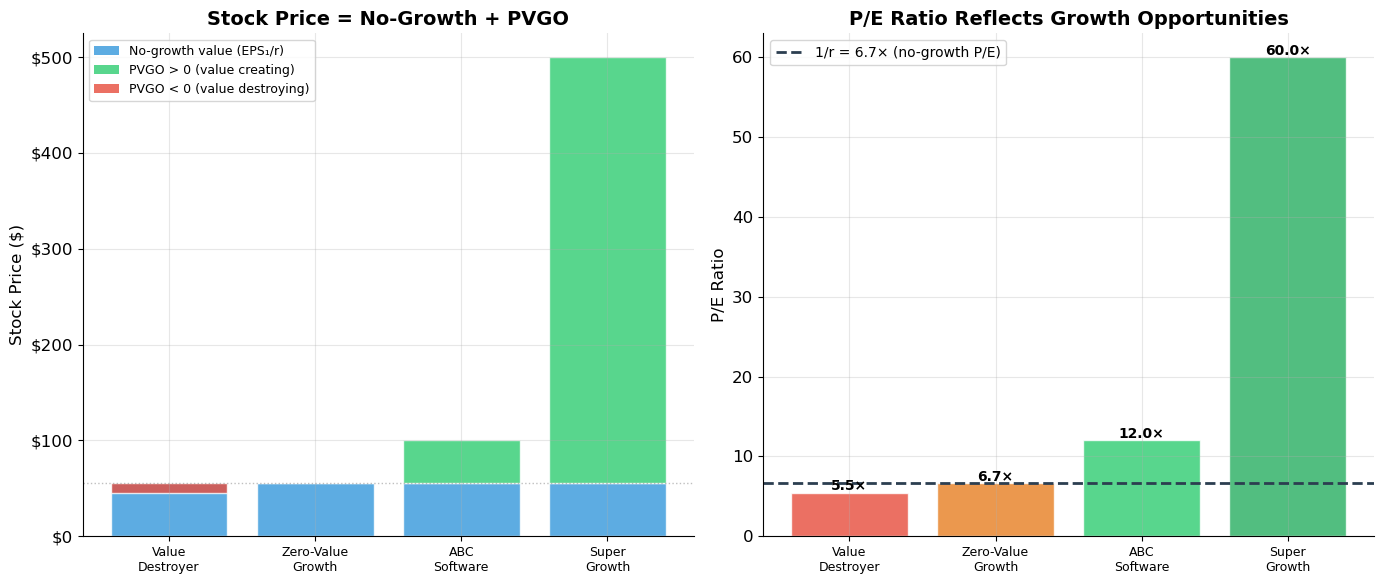
The PVGO Decomposition
Lo shows that any stock price can be decomposed into two components:
No-growth value (): the price if the firm distributed all earnings as dividends — no reinvestment, no growth
PVGO (Present Value of Growth Opportunities): the additional value created by reinvesting at returns above the cost of capital
When Does Growth Create Value?
Growth is valuable only when ROE > r — that is, when the firm can reinvest at a rate of return that exceeds what investors require.
If ROE = : PVGO = 0, and (the Texas Western result!)
If ROE < : PVGO < 0, and growth actually destroys value. The firm would be worth more if it stopped investing and paid out all earnings.
What Is a “Growth Stock”?
A growth stock is NOT merely a stock with growing EPS, growing dividends, or growing assets. It is a stock of a company with access to investments earning more than the cost of capital (ROE > ), so PVGO > 0.
Counterintuitively:
A stock with fast-growing EPS might NOT be a growth stock (if ROE < )
A stock with slow-growing EPS MIGHT be a growth stock (if ROE > )
The P/E Ratio and PVGO
Dividing both sides by :
This explains why high P/E ratios indicate growth stocks: P/E > 1/r implies PVGO > 0.
Source
# ============================================================
# Lo's ABC Software Example — PVGO Decomposition
# ============================================================
# From slide 18
EPS1_abc = 8.33
p_abc = 0.6        # payout ratio
ROE_abc = 0.25     # return on equity
r_abc = 0.15       # cost of capital

b_abc = 1 - p_abc  # plowback ratio = 0.4
g_abc = b_abc * ROE_abc  # sustainable growth = 10%
D1_abc = EPS1_abc * p_abc

print("=" * 65)
print("ABC SOFTWARE — Growth Opportunities (Lo's Example)")
print("=" * 65)
print(f"EPS₁ = ${EPS1_abc:.2f},  payout = {p_abc:.0%},  ROE = {ROE_abc:.0%},  r = {r_abc:.0%}")
print(f"Plowback b = {b_abc:.1f},  g = b × ROE = {b_abc:.1f} × {ROE_abc:.0%} = {g_abc:.0%}")
print(f"D₁ = EPS × p = ${D1_abc:.2f}")

# No-growth value
P0_nogrowth = EPS1_abc / r_abc
print(f"\nNo-growth value: EPS₁/r = ${EPS1_abc:.2f}/{r_abc:.2f} = ${P0_nogrowth:.2f}")

# Growth value
P0_growth = D1_abc / (r_abc - g_abc)
print(f"Growth value:    D₁/(r-g) = ${D1_abc:.2f}/({r_abc:.2f}-{g_abc:.2f}) = ${P0_growth:.2f}")

PVGO = P0_growth - P0_nogrowth
print(f"\nPVGO = P₀(growth) - P₀(no-growth) = ${P0_growth:.2f} - ${P0_nogrowth:.2f} = ${PVGO:.2f}")
print(f"PVGO share: {PVGO/P0_growth*100:.1f}% of stock price")

# Verify PVGO via NPV of growth investments
# At t=1: invest b*EPS = 0.4*8.33 = 3.33 at ROE=25% → perpetual CF of 0.25*3.33 = 0.83
inv_1 = b_abc * EPS1_abc
cf_from_inv1 = ROE_abc * inv_1
NPV_1 = -inv_1 + cf_from_inv1 / r_abc  # NPV at t=1

# PVGO = NPV_1 / (r - g) as a growing perpetuity
PVGO_check = NPV_1 / (r_abc - g_abc)

print(f"\nVerification via NPV of growth investments:")
print(f"  Year 1 investment: ${inv_1:.2f} at ROE={ROE_abc:.0%}")
print(f"  Perpetual CF from investment: ${cf_from_inv1:.2f}/year")
print(f"  NPV at t=1: -${inv_1:.2f} + ${cf_from_inv1:.2f}/{r_abc:.2f} = ${NPV_1:.2f}")
print(f"  PVGO = NPV₁/(r-g) = ${NPV_1:.2f}/({r_abc:.2f}-{g_abc:.2f}) = ${PVGO_check:.2f} ✓")
=================================================================
ABC SOFTWARE — Growth Opportunities (Lo's Example)
=================================================================
EPS₁ = $8.33, payout = 60%, ROE = 25%, r = 15%
Plowback b = 0.4, g = b × ROE = 0.4 × 25% = 10%
D₁ = EPS × p = $5.00
No-growth value: EPS₁/r = $8.33/0.15 = $55.53
Growth value: D₁/(r-g) = $5.00/(0.15-0.10) = $99.96
PVGO = P₀(growth) - P₀(no-growth) = $99.96 - $55.53 = $44.43
PVGO share: 44.4% of stock price
Verification via NPV of growth investments:
Year 1 investment: $3.33 at ROE=25%
Perpetual CF from investment: $0.83/year
NPV at t=1: -$3.33 + $0.83/0.15 = $2.22
PVGO = NPV₁/(r-g) = $2.22/(0.15-0.10) = $44.43 ✓
Source
# ============================================================
# PVGO Decomposition — Visualization
# ============================================================

def pvgo_decomposition(EPS1, r, ROE, b):
    """Compute price, no-growth value, and PVGO."""
    g = b * ROE
    D1 = EPS1 * (1 - b)
    if r <= g:
        return float('inf'), EPS1/r, float('inf'), g
    P0 = D1 / (r - g)
    P_nogrowth = EPS1 / r
    PVGO = P0 - P_nogrowth
    return P0, P_nogrowth, PVGO, g

# Compare firms with different ROE
firms = [
    ('Value Destroyer',  8.33, 0.15, 0.10, 0.4),  # ROE < r
    ('Zero-Value Growth', 8.33, 0.15, 0.15, 0.4),  # ROE = r
    ('ABC Software',     8.33, 0.15, 0.25, 0.4),   # ROE > r
    ('Super Growth',     8.33, 0.15, 0.35, 0.4),   # ROE >> r
]

fig, (ax1, ax2) = plt.subplots(1, 2, figsize=(14, 6))

names = []
no_growth_vals = []
pvgo_vals = []
pe_ratios = []

print("=" * 80)
print("PVGO DECOMPOSITION ACROSS FIRMS (all: EPS₁=$8.33, r=15%, b=0.4)")
print("=" * 80)
print(f"{'Firm':>20s} {'ROE':>6s} {'g':>6s} {'P₀':>8s} {'EPS/r':>8s} {'PVGO':>8s} {'P/E':>6s} {'PVGO%':>7s}")
print("-" * 80)

for name, eps, r, roe, b in firms:
    P0, P_ng, pvgo, g = pvgo_decomposition(eps, r, roe, b)
    pe = P0 / eps
    names.append(name.replace(' ', '\n'))
    no_growth_vals.append(P_ng)
    pvgo_vals.append(pvgo)
    pe_ratios.append(pe)
    print(f"{name:>20s} {roe:>6.0%} {g:>6.0%} ${P0:>7.2f} ${P_ng:>7.2f} ${pvgo:>+7.2f} {pe:>6.1f} {pvgo/P0*100:>6.1f}%")

# Left: Stacked bar chart
x = np.arange(len(names))
ax1.bar(x, no_growth_vals, color='#3498db', alpha=0.8, label='No-growth (EPS₁/r)', edgecolor='white')
for i, pv in enumerate(pvgo_vals):
    color = '#2ecc71' if pv >= 0 else '#e74c3c'
    ax1.bar(x[i], pv, bottom=no_growth_vals[i], color=color, alpha=0.8, edgecolor='white')

# Custom legend
from matplotlib.patches import Patch
legend_elements = [Patch(facecolor='#3498db', alpha=0.8, label='No-growth value (EPS₁/r)'),
                   Patch(facecolor='#2ecc71', alpha=0.8, label='PVGO > 0 (value creating)'),
                   Patch(facecolor='#e74c3c', alpha=0.8, label='PVGO < 0 (value destroying)')]
ax1.legend(handles=legend_elements, fontsize=9, loc='upper left')

ax1.set_xticks(x)
ax1.set_xticklabels(names, fontsize=9)
ax1.set_ylabel('Stock Price ($)', fontsize=12)
ax1.set_title('Stock Price = No-Growth + PVGO', fontsize=14, fontweight='bold')
ax1.axhline(y=no_growth_vals[0], color='gray', linewidth=1, linestyle=':', alpha=0.5)
ax1.yaxis.set_major_formatter(mticker.FuncFormatter(lambda x, _: f'${x:.0f}'))

# Right: P/E ratio
colors_pe = ['#e74c3c', '#e67e22', '#2ecc71', '#27ae60']
ax2.bar(x, pe_ratios, color=colors_pe, alpha=0.8, edgecolor='white')
ax2.axhline(y=1/0.15, color='#2c3e50', linewidth=2, linestyle='--',
            label=f'1/r = {1/0.15:.1f}× (no-growth P/E)')
ax2.set_xticks(x)
ax2.set_xticklabels(names, fontsize=9)
ax2.set_ylabel('P/E Ratio', fontsize=12)
ax2.set_title('P/E Ratio Reflects Growth Opportunities', fontsize=14, fontweight='bold')
ax2.legend(fontsize=10)

for i, pe in enumerate(pe_ratios):
    ax2.text(i, pe + 0.3, f'{pe:.1f}×', ha='center', fontsize=10, fontweight='bold')

plt.tight_layout()
plt.show()
================================================================================
PVGO DECOMPOSITION ACROSS FIRMS (all: EPS₁=$8.33, r=15%, b=0.4)
================================================================================
Firm ROE g P₀ EPS/r PVGO P/E PVGO%
--------------------------------------------------------------------------------
Value Destroyer 10% 4% $ 45.44 $ 55.53 $ -10.10 5.5 -22.2%
Zero-Value Growth 15% 6% $ 55.53 $ 55.53 $ +0.00 6.7 0.0%
ABC Software 25% 10% $ 99.96 $ 55.53 $ +44.43 12.0 44.4%
Super Growth 35% 14% $ 499.80 $ 55.53 $+444.27 60.0 88.9%
Source
# ============================================================
# When Does Growth Create/Destroy Value? — ROE vs. r
# ============================================================
EPS1 = 8.33
r = 0.15
b = 0.4

ROE_range = np.linspace(0.01, 0.40, 200)
prices = []
pvgos = []
pes = []

for roe in ROE_range:
    g = b * roe
    if r > g:
        D1 = EPS1 * (1 - b)
        P0 = D1 / (r - g)
        pvgo = P0 - EPS1/r
        prices.append(P0)
        pvgos.append(pvgo)
        pes.append(P0/EPS1)
    else:
        prices.append(np.nan)
        pvgos.append(np.nan)
        pes.append(np.nan)

fig, (ax1, ax2) = plt.subplots(1, 2, figsize=(14, 6))

# Left: PVGO vs ROE
ax1.plot(ROE_range * 100, pvgos, color='#2c3e50', linewidth=3)
ax1.axhline(y=0, color='#e74c3c', linewidth=2, linestyle='--')
ax1.axvline(x=r * 100, color='#e67e22', linewidth=2, linestyle=':', alpha=0.7)
ax1.fill_between(ROE_range * 100, 0, pvgos, where=np.array(pvgos) > 0,
                alpha=0.15, color='#2ecc71', label='PVGO > 0 (growth creates value)')
ax1.fill_between(ROE_range * 100, 0, pvgos, where=np.array(pvgos) < 0,
                alpha=0.15, color='#e74c3c', label='PVGO < 0 (growth destroys value)')

ax1.annotate(f'ROE = r = {r:.0%}\n(breakeven)', xy=(r*100, 0), xytext=(r*100 + 5, -15),
            fontsize=10, color='#e67e22', fontweight='bold',
            arrowprops=dict(arrowstyle='->', color='#e67e22', lw=1.5))

ax1.set_xlabel('Return on Equity (ROE) %', fontsize=12)
ax1.set_ylabel('PVGO ($)', fontsize=12)
ax1.set_title('PVGO vs. ROE\n(r = 15%, b = 0.4)', fontsize=14, fontweight='bold')
ax1.legend(fontsize=9)

# Right: P/E vs ROE
ax2.plot(ROE_range * 100, pes, color='#2c3e50', linewidth=3)
ax2.axhline(y=1/r, color='#e67e22', linewidth=2, linestyle='--', label=f'1/r = {1/r:.1f}× (no-growth P/E)')
ax2.axvline(x=r * 100, color='#e67e22', linewidth=1, linestyle=':', alpha=0.5)

ax2.set_xlabel('Return on Equity (ROE) %', fontsize=12)
ax2.set_ylabel('P/E Ratio', fontsize=12)
ax2.set_title('P/E Ratio vs. ROE\n(r = 15%, b = 0.4)', fontsize=14, fontweight='bold')
ax2.legend(fontsize=10)
ax2.set_ylim(0, 30)

plt.tight_layout()
plt.show()

print("Critical insight:")
print("• ROE > r: Growth creates value → PVGO > 0 → P/E > 1/r (growth stock)")
print("• ROE = r: Growth is value-neutral → PVGO = 0 → P/E = 1/r")
print("• ROE < r: Growth DESTROYS value → PVGO < 0 → P/E < 1/r")
print("\nA 'growth stock' is defined by ROE > r, NOT by growing EPS!")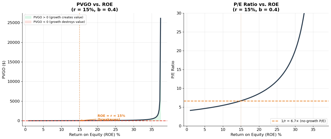
Critical insight:
• ROE > r: Growth creates value → PVGO > 0 → P/E > 1/r (growth stock)
• ROE = r: Growth is value-neutral → PVGO = 0 → P/E = 1/r
• ROE < r: Growth DESTROYS value → PVGO < 0 → P/E < 1/r

A 'growth stock' is defined by ROE > r, NOT by growing EPS!
8. Exercises
Exercise 1: Gordon Growth Model
A utility company just paid a dividend of $3.50 per share. Dividends are expected to grow at 3% per year indefinitely.
(a) If the required return is 9%, what is the stock price?
(b) If the stock is currently trading at $65, what cost of equity is the market implying?
(c) If management announces it will increase the growth rate to 5% by reducing the payout ratio, but the required return also increases to 11% due to higher risk, what happens to the stock price? Is the growth strategy value-creating?
(d) The CEO claims “our stock is undervalued because the market doesn’t understand our growth.” If the current price is $55 and r = 9%, what growth rate is the market implying? Is the CEO’s claim plausible if ROE = 12%?
Source
# Exercise 1 — Workspace
# D0 = 3.50; g = 0.03; r = 0.09
#
# (a) P0 = D0*(1+g)/(r-g) = 3.50*1.03/(0.09-0.03)
# P0 = ?
#
# (b) Trading at $65: r = D1/P0 + g = 3.50*1.03/65 + 0.03
# r = ?
#
# (c) New g=0.05, new r=0.11
# P0_new = 3.50*(1.05)/(0.11-0.05)
# Compare with original
#
# (d) 55 = 3.50*(1+g)/(0.09-g)  →  solve for g
# from scipy.optimize import brentq
# g_implied = brentq(lambda g: 3.50*(1+g)/(0.09-g) - 55, 0, 0.089)
# print(f"Implied g = {g_implied:.2%}")
Exercise 2: Two-Stage Growth Model
TechCorp has just paid a dividend of $1.20. Analysts expect 20% dividend growth for the next 5 years, followed by 4% growth forever. The cost of equity is 14%.
(a) Compute the stock price using the two-stage DDM.
(b) What fraction of the stock’s value comes from the terminal value? Why is this fraction typically so large?
(c) If the market prices the stock at $35, what stable growth rate is being implied (keeping all else equal)? Use numerical methods.
(d) Run a sensitivity analysis: how does the stock price change as varies from 2% to 6% and as varies from 12% to 16%? Present your results as a table.
Source
# Exercise 2 — Workspace
# D0, r, g_H, T, g_L = 1.20, 0.14, 0.20, 5, 0.04
#
# (a)
# pv1, pv2, P0 = two_stage_ddm(D0, r, g_H, T, g_L)
# print(f"P₀ = ${P0:.2f}")
#
# (b)
# print(f"Terminal value share: {pv2/(pv1+pv2)*100:.1f}%")
#
# (c) Find g_L such that P0 = 35
# g_implied = brentq(lambda g: two_stage_ddm(D0, r, g_H, T, g)[2] - 35, 0, 0.139)
# print(f"Implied g_L = {g_implied:.2%}")
Exercise 3: PVGO and Growth Stocks
MegaCorp has: EPS₁ = $5.00, payout ratio = 50%, ROE = 18%, cost of equity = 12%.
(a) Compute the sustainable growth rate, dividend, stock price, and P/E ratio.
(b) Decompose the stock price into no-growth value and PVGO. What fraction of value comes from growth opportunities?
(c) A competitor, SteadyCorp, has the same EPS and cost of equity but ROE = 12% (equal to ). It also retains 50%. Compute SteadyCorp’s price, PVGO, and P/E. What happens if SteadyCorp increases retention to 80%?
(d) A value investor argues: “I only buy stocks with P/E < 10. High P/E stocks are overpriced.” Using the PVGO framework, explain why this rule might cause the investor to miss excellent opportunities. When might the rule be correct?
Source
# Exercise 3 — Workspace
# EPS1, p, ROE, r = 5.00, 0.50, 0.18, 0.12
# b = 1 - p
# g = b * ROE
# D1 = EPS1 * p
# P0 = D1 / (r - g)
# P_nogrowth = EPS1 / r
# PVGO = P0 - P_nogrowth
# PE = P0 / EPS1
#
# print(f"g = {g:.2%}, D₁ = ${D1:.2f}")
# print(f"P₀ = ${P0:.2f}, P/E = {PE:.1f}×")
# print(f"No-growth: ${P_nogrowth:.2f}, PVGO: ${PVGO:.2f} ({PVGO/P0*100:.1f}%)")
Key Takeaways — Session 6
The DDM values a stock as the present value of all future dividends: . The holding period doesn’t matter — the price reflects the infinite dividend stream.
The Gordon Growth Model is the workhorse of equity valuation. It requires and is extremely sensitive to the spread .
Cost of equity can be estimated from the DDM: (dividend yield + growth). Returns decompose into income (dividends) and capital gains (growth).
Multi-stage models handle firms transitioning from high to stable growth. The terminal value (stable phase) typically dominates, accounting for 60–80% of total value.
Sustainable growth . The link between dividends and earnings is through the payout ratio.
Stock price = No-growth value + PVGO. Growth creates value only when ROE > . A true “growth stock” is defined by having PVGO > 0, not by having fast-growing EPS.
P/E ratio = + PVGO/EPS. High P/E signals growth opportunities. P/E equals only when the firm earns exactly its cost of capital on new investments.
References
Brealey, R.A., Myers, S.C., and Allen, F. Principles of Corporate Finance, Chapter 4.
MIT OCW 15.401: Equities
Gordon, M.J. (1959). “Dividends, Earnings, and Stock Prices.” Review of Economics and Statistics, 41(2), 99–105.
Harris, L. (2002). Trading and Exchanges: Market Microstructure for Practitioners. Oxford University Press.
Malkiel, B. (1996). A Random Walk Down Wall Street. W.W. Norton.
Next: Session 7 — Forward and Futures Contracts — forward pricing, cost of carry, futures markets, and hedging applications.