Lecture 2: Present Value Relations I
MIT 15.401 — Finance Theory I (Prof. Andrew Lo)
Video: MIT OCW — Part I of Present Value Relations
Readings: Brealey, Myers, and Allen — Chapters 2–3
This notebook covers Session 2 — arguably the most foundational lecture in the entire course. It develops the Present Value (PV) operator, the single most important tool in all of finance. Every valuation problem ultimately reduces to a present value calculation.
We cover the definition of an asset as a sequence of cash flows, the time value of money, the NPV rule, and the special cash flow patterns (perpetuities and annuities) that appear throughout finance.
Table of Contents
Source
# ============================================================
# Setup
# ============================================================
import numpy as np
import pandas as pd
import matplotlib.pyplot as plt
import matplotlib.ticker as mticker
from IPython.display import display, Markdown

plt.rcParams.update({
    'figure.figsize': (10, 5),
    'axes.spines.top': False,
    'axes.spines.right': False,
    'axes.grid': True,
    'grid.alpha': 0.3,
    'font.size': 12,
    'lines.linewidth': 2,
})
print("Libraries loaded successfully.")
Libraries loaded successfully.
1. Cash Flows and the Definition of an Asset
An asset is any sequence of cash flows.
| Example | Cash Flow Sequence |
|---|---|
| A bond | Fixed coupon payments + face value at maturity |
| A stock | Stream of uncertain future dividends |
| A business | Net cash flows from operations |
| A rental property | Monthly rent payments minus expenses |
| Your career | Lifetime stream of salary income |
Formally:
The Currency Analogy
Cash flows at different points in time are like cash in different currencies. The discount rate is the exchange rate that converts future dollars into present dollars — a single numéraire (dollars at time 0).
Source
# ============================================================
# Cash Flow Timeline Visualization
# ============================================================

def plot_cashflow_timeline(cashflows, title="Cash Flow Timeline", discount_rate=None):
    """Visualize cash flows on a timeline, optionally showing PVs."""
    times = sorted(cashflows.keys())
    cfs = [cashflows[t] for t in times]
    max_abs = max(abs(c) for c in cfs)

    fig, ax = plt.subplots(figsize=(12, 5))
    ax.axhline(y=0, color='#2c3e50', linewidth=2, zorder=1)

    for t, cf in zip(times, cfs):
        color = '#2ecc71' if cf >= 0 else '#e74c3c'
        ax.bar(t, cf, width=0.4, color=color, alpha=0.85, edgecolor='white', linewidth=2, zorder=2)
        offset = 0.05 * max_abs * (1 if cf >= 0 else -1)
        ax.text(t, cf + offset, f'${cf:+,.0f}', ha='center',
                va='bottom' if cf >= 0 else 'top', fontsize=11, fontweight='bold', color=color)

    if discount_rate is not None:
        pvs = [cf / (1 + discount_rate)**t for t, cf in zip(times, cfs)]
        for t, cf, pv in zip(times, cfs, pvs):
            if t > 0:
                ax.annotate(f'PV = ${pv:,.0f}', xy=(t, 0),
                           xytext=(t, -0.25 * max_abs), fontsize=9, ha='center',
                           color='#8e44ad', style='italic',
                           arrowprops=dict(arrowstyle='->', color='#8e44ad', lw=1))
        npv = sum(pvs)
        ax.text(0.98, 0.25, f'NPV = ${npv:,.0f}\n(r = {discount_rate:.0%})',
                transform=ax.transAxes, ha='right', va='top', fontsize=13,
                fontweight='bold', color='#8e44ad',
                bbox=dict(boxstyle='round,pad=0.5', facecolor='#f4ecf7', alpha=0.9))

    for t in times:
        ax.plot(t, 0, 'o', color='#2c3e50', markersize=8, zorder=3)

    ax.set_xlabel('Time Period (t)', fontsize=13)
    ax.set_ylabel('Cash Flow ($)', fontsize=13)
    ax.set_title(title, fontsize=14, fontweight='bold')
    ax.set_xticks(times)
    ax.set_xticklabels([f't={t}' for t in times])
    ax.yaxis.set_major_formatter(mticker.FuncFormatter(lambda x, _: f'${x:,.0f}'))
    ax.set_ylim(-300000,200000)
    plt.tight_layout()
    plt.show()


# Lo's lecture example
plot_cashflow_timeline({0: -230000, 1: 90000, 2: 90000, 3: 90000},
                       title="Example: Capital Investment Project (Lo's Lecture)",
                       discount_rate=0.04)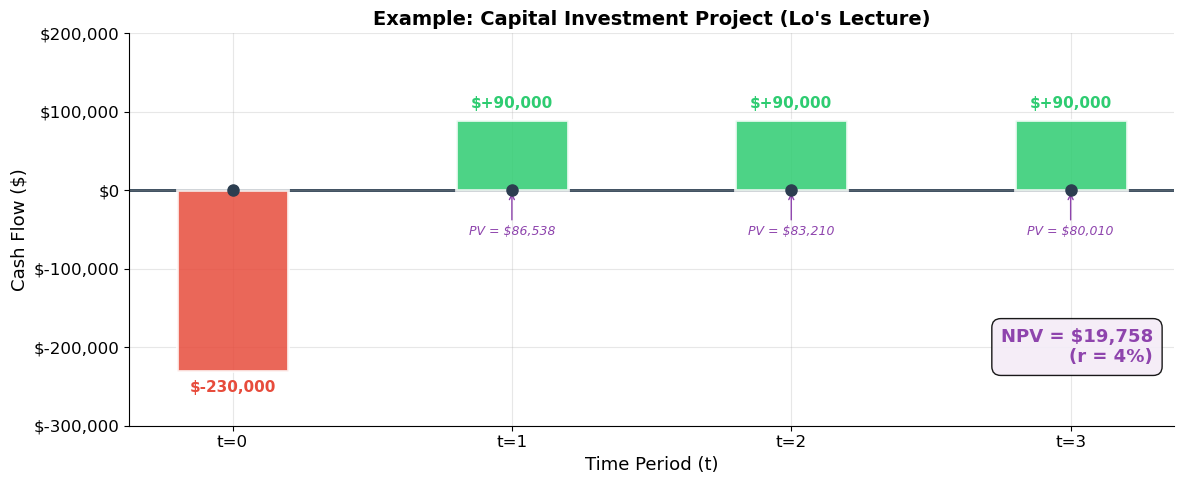
2. The Present Value Operator
Forward (compounding):
Backward (discounting):
Key Properties
Linearity:
Only relative time matters:
Discount factor < 1 for
Assumptions (to be relaxed later)
Cash flows and rates are known with certainty
No transaction costs
Constant discount rate
Source
# ============================================================
# Discount Factor Decay
# ============================================================
periods = np.arange(0, 51)
rates = [0.01, 0.03, 0.05, 0.08, 0.10, 0.15]
colors = ['#27ae60', '#2ecc71', '#3498db', '#e67e22', '#e74c3c', '#8e44ad']

fig, (ax1, ax2) = plt.subplots(1, 2, figsize=(14, 6))

for r, color in zip(rates, colors):
    ax1.plot(periods, 1 / (1 + r)**periods, label=f'r = {r:.0%}', color=color, linewidth=2)

ax1.set_xlabel('Periods (n)')
ax1.set_ylabel('Discount Factor  1/(1+r)ⁿ')
ax1.set_title('Discount Factor Decay Over Time', fontsize=14, fontweight='bold')
ax1.legend(fontsize=10)
ax1.set_ylim(0, 1.05)
ax1.axhline(y=0.5, color='gray', linestyle=':', alpha=0.5)

horizons = [1, 5, 10, 20, 30, 50]
rate_range = np.linspace(0.01, 0.15, 100)
cmap = plt.cm.viridis
for i, T in enumerate(horizons):
    ax2.plot(rate_range * 100, 1000 / (1 + rate_range)**T,
            label=f'T = {T} yrs', color=cmap(i / len(horizons)), linewidth=2)

ax2.set_xlabel('Discount Rate (%)')
ax2.set_ylabel('Present Value ($)')
ax2.set_title('PV of $1,000 at Various Horizons', fontsize=14, fontweight='bold')
ax2.yaxis.set_major_formatter(mticker.FuncFormatter(lambda x, _: f'${x:,.0f}'))
ax2.legend(fontsize=10)

plt.tight_layout()
plt.show()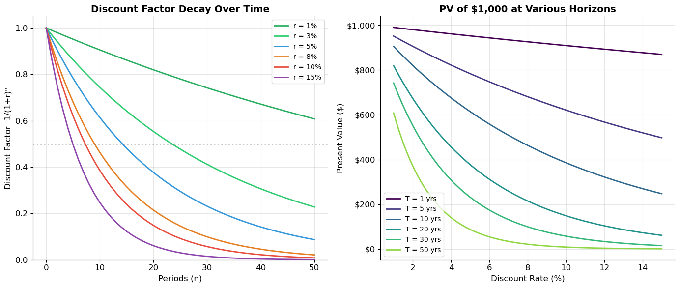
3. The Time Value of Money
A dollar today > a dollar tomorrow. Three reasons: opportunity cost, impatience, inflation.
Source
# ============================================================
# NPV Calculation — Lo's Worked Example
# ============================================================

def compute_npv(cashflows, rate):
    """Compute NPV of a cash flow sequence."""
    return sum(cf / (1 + rate)**t for t, cf in enumerate(cashflows))

cashflows = [-230_000, 90_000, 90_000, 90_000]
r = 0.04

print("=" * 65)
print("NPV CALCULATION — Lo's Capital Investment Example")
print("=" * 65)
for t, cf in enumerate(cashflows):
    df = 1 / (1 + r)**t
    pv = cf * df
    print(f"  t={t}:  CF = ${cf:>10,.0f}  ×  1/(1.04)^{t} = {df:.6f}  →  PV = ${pv:>10,.2f}")
print("-" * 65)
npv = compute_npv(cashflows, r)
print(f"  NPV = ${npv:,.2f}")
print(f"  Decision: {'✅ ACCEPT' if npv > 0 else '❌ REJECT'}")
=================================================================
NPV CALCULATION — Lo's Capital Investment Example
=================================================================
t=0: CF = $ -230,000 × 1/(1.04)^0 = 1.000000 → PV = $-230,000.00
t=1: CF = $ 90,000 × 1/(1.04)^1 = 0.961538 → PV = $ 86,538.46
t=2: CF = $ 90,000 × 1/(1.04)^2 = 0.924556 → PV = $ 83,210.06
t=3: CF = $ 90,000 × 1/(1.04)^3 = 0.888996 → PV = $ 80,009.67
-----------------------------------------------------------------
NPV = $19,758.19
Decision: ✅ ACCEPT
Source
# ============================================================
# NPV Profile — NPV as a function of discount rate
# ============================================================
# ▶ MODIFY CASH FLOWS HERE AND RE-RUN
cashflows = [-230_000, 90_000, 90_000, 90_000]
# ============================================================

rates = np.linspace(0.001, 0.30, 300)
npvs = [compute_npv(cashflows, r) for r in rates]

fig, ax = plt.subplots(figsize=(11, 6))
ax.plot(rates * 100, npvs, color='#2c3e50', linewidth=3)
ax.axhline(y=0, color='#e74c3c', linewidth=1.5, linestyle='--', alpha=0.7)
ax.fill_between(rates * 100, npvs, 0, where=np.array(npvs) > 0, alpha=0.15, color='#2ecc71', label='NPV > 0 (Accept)')
ax.fill_between(rates * 100, npvs, 0, where=np.array(npvs) < 0, alpha=0.15, color='#e74c3c', label='NPV < 0 (Reject)')

# Find IRR
for i in range(len(npvs) - 1):
    if npvs[i] * npvs[i+1] < 0:
        irr = rates[i] + (rates[i+1] - rates[i]) * npvs[i] / (npvs[i] - npvs[i+1])
        ax.plot(irr * 100, 0, 'o', color='#e74c3c', markersize=12, zorder=5)
        ax.annotate(f'IRR = {irr:.2%}', xy=(irr*100, 0), xytext=(irr*100 + 3, max(npvs)*0.3),
                   fontsize=13, fontweight='bold', color='#e74c3c',
                   arrowprops=dict(arrowstyle='->', color='#e74c3c', lw=2))
        break

ax.set_xlabel('Discount Rate (%)', fontsize=13)
ax.set_ylabel('Net Present Value ($)', fontsize=13)
ax.set_title('NPV Profile', fontsize=14, fontweight='bold')
ax.yaxis.set_major_formatter(mticker.FuncFormatter(lambda x, _: f'${x:,.0f}'))
ax.legend(fontsize=11)
plt.tight_layout()
plt.show()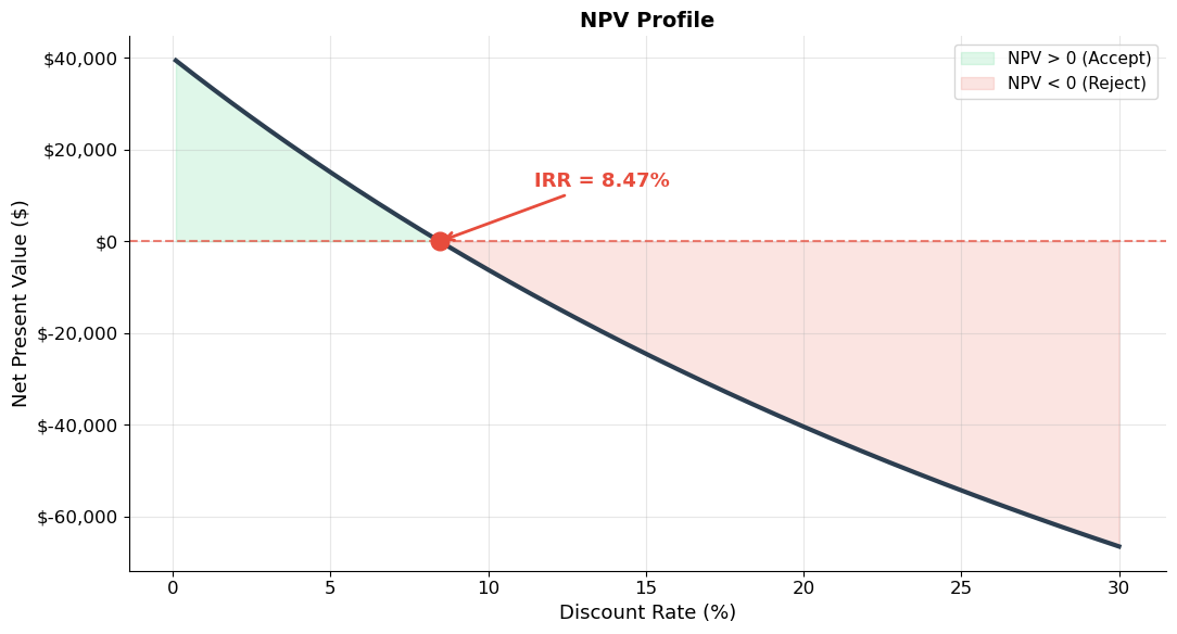
5. Special Cash Flows: The Perpetuity
A perpetuity pays every period, forever. The geometric series gives:
Intuition: Depositing at rate earns per year forever without touching principal.
Source
# ============================================================
# Perpetuity: Partial Sums Converging to C/r
# ============================================================
# ▶ MODIFY AND RE-RUN
C = 100    # Annual payment
r = 0.05   # Discount rate
# ============================================================

exact_pv = C / r
max_terms = 150
terms = np.arange(1, max_terms + 1)
partial_sums = np.cumsum([C / (1 + r)**t for t in terms])
pct_captured = partial_sums / exact_pv * 100

fig, (ax1, ax2) = plt.subplots(1, 2, figsize=(14, 6))

ax1.plot(terms, partial_sums, color='#3498db', linewidth=2.5, label='Partial sum')
ax1.axhline(y=exact_pv, color='#e74c3c', linewidth=2, linestyle='--', label=f'C/r = ${exact_pv:,.0f}')
ax1.fill_between(terms, partial_sums, exact_pv, alpha=0.1, color='#e74c3c')

for pct_target in [90, 95, 99]:
    idx = np.argmax(pct_captured >= pct_target)
    ax1.plot(terms[idx], partial_sums[idx], 'o', color='#2ecc71', markersize=8, zorder=5)
    ax1.annotate(f'{pct_target}% at t={terms[idx]}', xy=(terms[idx], partial_sums[idx]),
                xytext=(terms[idx]+10, partial_sums[idx] - exact_pv*0.08), fontsize=9, color='#27ae60',
                arrowprops=dict(arrowstyle='->', color='#27ae60', lw=1))

ax1.set_xlabel('Number of Terms')
ax1.set_ylabel('Present Value ($)')
ax1.set_title(f'Partial Sums → C/r  (C=${C}, r={r:.0%})', fontsize=14, fontweight='bold')
ax1.yaxis.set_major_formatter(mticker.FuncFormatter(lambda x, _: f'${x:,.0f}'))
ax1.legend(fontsize=11)

dcfs = [C / (1 + r)**t for t in range(1, 51)]
ax2.bar(range(1, 51), dcfs, color='#3498db', alpha=0.7, edgecolor='white')
ax2.set_xlabel('Period (t)')
ax2.set_ylabel('Discounted Cash Flow ($)')
ax2.set_title('Individual Discounted Cash Flows', fontsize=14, fontweight='bold')

plt.tight_layout()
plt.show()
print(f"Exact PV = C/r = {C}/{r} = ${exact_pv:,.2f}")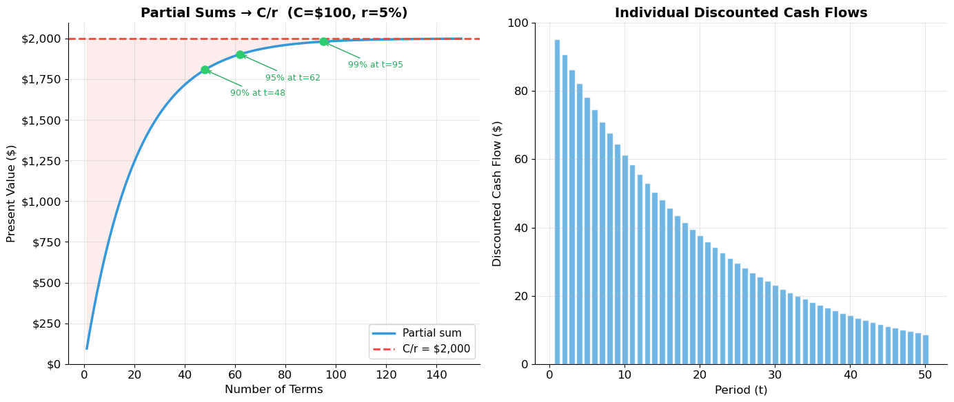
Exact PV = C/r = 100/0.05 = $2,000.00
6. Special Cash Flows: The Growing Perpetuity
Cash flows grow at constant rate :
This is the foundation of the Gordon Growth Model for stocks:
Source
# ============================================================
# Growing Perpetuity: Sensitivity to Growth Rate
# ============================================================
# ▶ MODIFY AND RE-RUN
C = 100
r = 0.08
# ============================================================

g_values = np.linspace(0, r - 0.005, 200)
pv_values = C / (r - g_values)

fig, (ax1, ax2) = plt.subplots(1, 2, figsize=(14, 6))

ax1.plot(g_values * 100, pv_values, color='#2c3e50', linewidth=3)
ax1.axhline(y=C/r, color='#3498db', linewidth=1.5, linestyle='--', label=f'No growth: C/r = ${C/r:,.0f}', alpha=0.7)
ax1.axvline(x=r*100, color='#e74c3c', linewidth=1.5, linestyle=':', label=f'Asymptote: g = r = {r:.0%}', alpha=0.7)
for g_mark in [0.02, 0.04, 0.06]:
    if g_mark < r:
        pv_mark = C / (r - g_mark)
        ax1.plot(g_mark*100, pv_mark, 'o', color='#2ecc71', markersize=8, zorder=5)
        ax1.annotate(f'g={g_mark:.0%}: ${pv_mark:,.0f}', xy=(g_mark*100, pv_mark),
                    xytext=(g_mark*100+0.5, pv_mark + max(pv_values)*0.02), fontsize=9)

ax1.set_xlabel('Growth Rate g (%)')
ax1.set_ylabel('Present Value ($)')
ax1.set_title('PV = C/(r−g)', fontsize=14, fontweight='bold')
ax1.yaxis.set_major_formatter(mticker.FuncFormatter(lambda x, _: f'${x:,.0f}'))
ax1.set_ylim(0, min(max(pv_values)*1.1, C/r*8))
ax1.legend(fontsize=10)

periods = np.arange(1, 31)
for g, color, ls in [(0, '#3498db', '--'), (0.02, '#2ecc71', '-'), (0.04, '#e67e22', '-'), (0.06, '#e74c3c', '-')]:
    if g < r:
        ax2.plot(periods, C*(1+g)**(periods-1) / (1+r)**periods, color=color, linewidth=2, linestyle=ls, label=f'g = {g:.0%}')
ax2.set_xlabel('Period')
ax2.set_ylabel('Discounted Cash Flow ($)')
ax2.set_title('DCFs Over Time', fontsize=14, fontweight='bold')
ax2.legend(fontsize=10)

plt.tight_layout()
plt.show()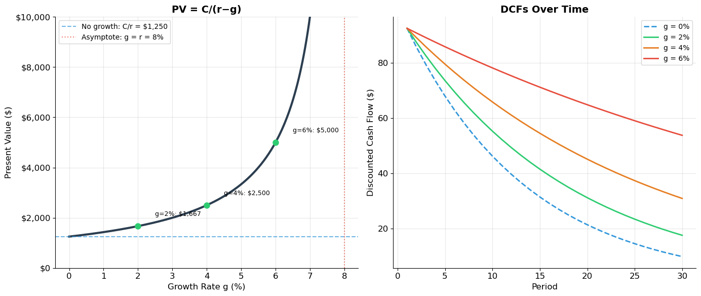
7. Special Cash Flows: The Annuity
An annuity pays for periods. Using the perpetuity difference trick:
Future value:
Source
# ============================================================
# Core PV Functions — Reusable Toolkit
# ============================================================

def pv_perpetuity(C, r):
    return C / r

def pv_growing_perpetuity(C, r, g):
    return C / (r - g) if r > g else float('inf')

def annuity_discount_factor(r, T):
    return (1 - (1 + r)**(-T)) / r if r != 0 else T

def pv_annuity(C, r, T):
    return C * annuity_discount_factor(r, T)

def fv_annuity(C, r, T):
    return C * ((1 + r)**T - 1) / r if r != 0 else C * T

def pv_growing_annuity(C, r, g, T):
    if abs(r - g) < 1e-10:
        return C * T / (1 + r)
    return C * (1 - ((1 + g) / (1 + r))**T) / (r - g)

# Verification
print("PV Formula Verification")
print("=" * 55)
print(f"Perpetuity ($100/yr, r=5%):          ${pv_perpetuity(100, 0.05):>10,.2f}")
print(f"Growing Perp ($100/yr, r=8%, g=3%):  ${pv_growing_perpetuity(100, 0.08, 0.03):>10,.2f}")
print(f"Annuity ($100/yr, r=5%, T=20):       ${pv_annuity(100, 0.05, 20):>10,.2f}")
print(f"ADF(5%, 20) =                        {annuity_discount_factor(0.05, 20):>10.6f}")

print(f"\nConvergence: annuity → perpetuity as T → ∞ (C=$100, r=5%):")
pv_p = pv_perpetuity(100, 0.05)
for T in [10, 20, 50, 100, 500]:
    pv_a = pv_annuity(100, 0.05, T)
    print(f"  T={T:>4d}: ${pv_a:>10,.2f}  ({pv_a/pv_p:.4%} of perpetuity)")
PV Formula Verification
=======================================================
Perpetuity ($100/yr, r=5%): $ 2,000.00
Growing Perp ($100/yr, r=8%, g=3%): $ 2,000.00
Annuity ($100/yr, r=5%, T=20): $ 1,246.22
ADF(5%, 20) = 12.462210
Convergence: annuity → perpetuity as T → ∞ (C=$100, r=5%):
T= 10: $ 772.17 (38.6087% of perpetuity)
T= 20: $ 1,246.22 (62.3111% of perpetuity)
T= 50: $ 1,825.59 (91.2796% of perpetuity)
T= 100: $ 1,984.79 (99.2396% of perpetuity)
T= 500: $ 2,000.00 (100.0000% of perpetuity)
Source
# ============================================================
# Annuity = Perpetuity − Delayed Perpetuity
# ============================================================
# ▶ MODIFY AND RE-RUN
C, r, T = 100, 0.05, 10
# ============================================================

periods = np.arange(1, T + 25)
perp1_dcf = np.array([C / (1 + r)**t for t in periods])
perp2_dcf = np.array([C / (1 + r)**t if t > T else 0 for t in periods])
annuity_dcf = np.array([C / (1 + r)**t if t <= T else 0 for t in periods])

fig, axes = plt.subplots(1, 3, figsize=(16, 5), sharey=True)

axes[0].bar(periods, perp1_dcf, color='#3498db', alpha=0.7, edgecolor='white')
axes[0].set_title(f'Perpetuity\nPV = ${C/r:,.0f}', fontsize=12, fontweight='bold')
axes[0].axvline(x=T+0.5, color='#e74c3c', linestyle='--', alpha=0.5)

pv_del = (C/r) / (1+r)**T
axes[1].bar(periods, perp2_dcf, color='#e74c3c', alpha=0.7, edgecolor='white')
axes[1].set_title(f'Delayed Perpetuity\nPV = ${pv_del:,.0f}', fontsize=12, fontweight='bold')
axes[1].axvline(x=T+0.5, color='#e74c3c', linestyle='--', alpha=0.5)

pv_ann = pv_annuity(C, r, T)
axes[2].bar(periods, annuity_dcf, color='#2ecc71', alpha=0.7, edgecolor='white')
axes[2].set_title(f'Annuity (T={T})\nPV = ${pv_ann:,.0f}', fontsize=12, fontweight='bold')
axes[2].axvline(x=T+0.5, color='#e74c3c', linestyle='--', alpha=0.5)

for ax in axes:
    ax.set_xlabel('Period')
axes[0].set_ylabel('Discounted CF ($)')
fig.suptitle(f'Annuity = Perpetuity − Delayed Perpetuity', fontsize=14, fontweight='bold', y=1.02)
plt.tight_layout()
plt.show()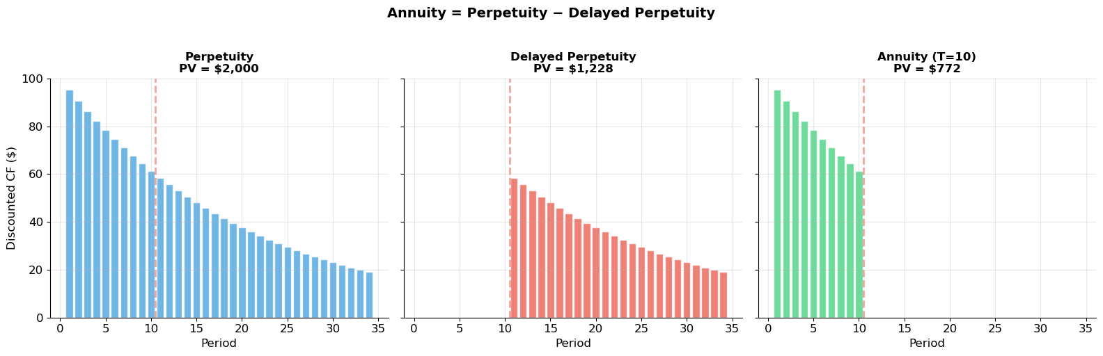
Source
# ============================================================
# Application: Mortgage Amortization
# ============================================================
# ▶ MODIFY AND RE-RUN
principal = 400_000
annual_rate = 0.06
years = 30
# ============================================================

monthly_rate = annual_rate / 12
n_payments = years * 12
monthly_payment = principal * monthly_rate / (1 - (1 + monthly_rate)**(-n_payments))

balance = principal
balances, interest_parts, principal_parts = [principal], [], []
total_interest = 0

for month in range(1, n_payments + 1):
    interest = balance * monthly_rate
    ppay = monthly_payment - interest
    balance -= ppay
    balances.append(max(balance, 0))
    interest_parts.append(interest)
    principal_parts.append(ppay)
    total_interest += interest

print("=" * 55)
print("MORTGAGE ANALYSIS")
print("=" * 55)
print(f"Loan amount:         ${principal:>12,.0f}")
print(f"Rate:                 {annual_rate:>11.2%}")
print(f"Term:                 {years:>8} years")
print(f"Monthly payment:     ${monthly_payment:>12,.2f}")
print(f"Total payments:      ${monthly_payment * n_payments:>12,.0f}")
print(f"Total interest:      ${total_interest:>12,.0f}")
print(f"Interest/Principal:   {total_interest/principal:>11.1%}")

annual_int = [sum(interest_parts[i*12:(i+1)*12]) for i in range(years)]
annual_prin = [sum(principal_parts[i*12:(i+1)*12]) for i in range(years)]

fig, (ax1, ax2) = plt.subplots(1, 2, figsize=(14, 6))

months = np.arange(0, n_payments + 1)
ax1.fill_between(months/12, balances, alpha=0.3, color='#3498db')
ax1.plot(months/12, balances, color='#3498db', linewidth=2.5)
ax1.set_xlabel('Year')
ax1.set_ylabel('Remaining Balance ($)')
ax1.set_title('Loan Balance Over Time', fontsize=14, fontweight='bold')
ax1.yaxis.set_major_formatter(mticker.FuncFormatter(lambda x, _: f'${x:,.0f}'))

yr = np.arange(1, years + 1)
ax2.bar(yr, annual_int, color='#e74c3c', alpha=0.8, label='Interest', edgecolor='white')
ax2.bar(yr, annual_prin, bottom=annual_int, color='#2ecc71', alpha=0.8, label='Principal', edgecolor='white')
ax2.set_xlabel('Year')
ax2.set_ylabel('Annual Payment ($)')
ax2.set_title('Interest vs. Principal', fontsize=14, fontweight='bold')
ax2.yaxis.set_major_formatter(mticker.FuncFormatter(lambda x, _: f'${x:,.0f}'))
ax2.legend(fontsize=11)

plt.tight_layout()
plt.show()
=======================================================
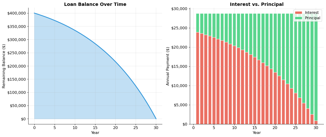
MORTGAGE ANALYSIS
=======================================================
Loan amount: $ 400,000
Rate: 6.00%
Term: 30 years
Monthly payment: $ 2,398.20
Total payments: $ 863,353
Total interest: $ 463,353
Interest/Principal: 115.8%
Source
# ============================================================
# Compounding Frequency and Effective Annual Rate
# ============================================================
# ▶ MODIFY AND RE-RUN
stated_rate = 0.10
# ============================================================
frequencies = {'Annual': 1, 'Semi-annual': 2, 'Quarterly': 4,
'Monthly': 12, 'Weekly': 52, 'Daily': 365}
continuous_ear = np.exp(stated_rate) - 1
print(f"Stated (nominal) annual rate: {stated_rate:.2%}")
print("=" * 55)
print(f"{'Compounding':15s} {'n':>5s} {'EAR':>12s} {'vs stated':>10s}")
print("-" * 55)
names, ears = [], []
for name, n in frequencies.items():
ear = (1 + stated_rate / n)**n - 1
print(f"{name:15s} {n:>5d} {ear:>12.6%} {ear - stated_rate:>+10.6%}")
names.append(name)
ears.append(ear)
print(f"{'Continuous':15s} {'∞':>5s} {continuous_ear:>12.6%} {continuous_ear - stated_rate:>+10.6%}")
names.append('Continuous')
ears.append(continuous_ear)
fig, (ax1, ax2) = plt.subplots(1, 2, figsize=(14, 5))
colors = ['#3498db'] * len(names)
colors[-1] = '#e74c3c'
ax1.barh(names, [e*100 for e in ears], color=colors, alpha=0.8, edgecolor='white')
ax1.axvline(x=stated_rate*100, color='#2c3e50', linewidth=2, linestyle='--', label=f'Stated = {stated_rate:.0%}')
ax1.set_xlabel('EAR (%)')
ax1.set_title('EAR by Compounding Frequency', fontsize=14, fontweight='bold')
ax1.legend(fontsize=10)
ax1.invert_yaxis()
n_range = np.arange(1, 366)
ax2.plot(n_range, ((1 + stated_rate/n_range)**n_range - 1)*100, color='#3498db', linewidth=2.5)
ax2.axhline(y=continuous_ear*100, color='#e74c3c', linewidth=1.5, linestyle='--', label=f'Continuous = {continuous_ear:.4%}')
ax2.set_xlabel('Compounding Frequency (n)')
ax2.set_ylabel('EAR (%)')
ax2.set_title('Convergence to Continuous Limit', fontsize=14, fontweight='bold')
ax2.legend(fontsize=10)
ax2.set_xscale('log')
plt.tight_layout()
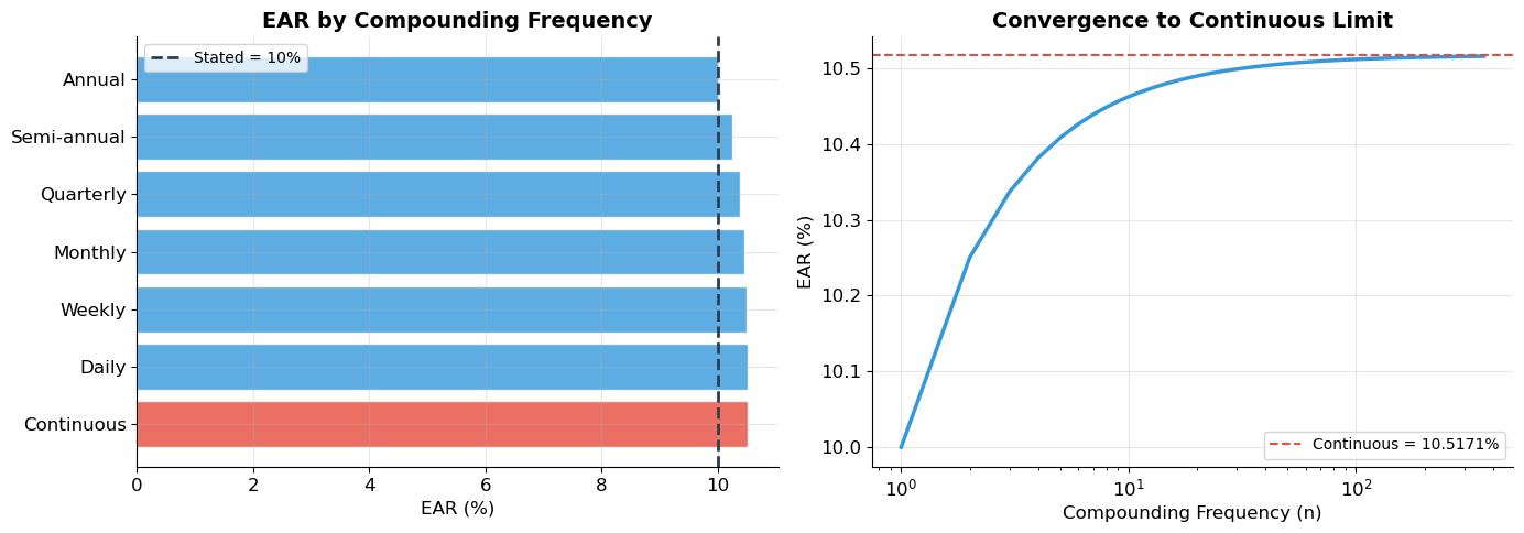
plt.show()Stated (nominal) annual rate: 10.00%
=======================================================
Compounding n EAR vs stated
-------------------------------------------------------
Annual 1 10.000000% +0.000000%
Semi-annual 2 10.250000% +0.250000%
Quarterly 4 10.381289% +0.381289%
Monthly 12 10.471307% +0.471307%
Weekly 52 10.506479% +0.506479%
Daily 365 10.515578% +0.515578%
Continuous ∞ 10.517092% +0.517092%
Summary of Key Formulas
| Formula | Expression | Conditions |
|---|---|---|
| Future Value | — | |
| Present Value | — | |
| NPV | Accept if NPV > 0 | |
| Perpetuity | ||
| Growing Perpetuity | ||
| Annuity | — | |
| Growing Annuity | ||
| EAR | — | |
| Continuous | — |
9. Exercises
Exercise 1: NPV Investment Decision
A property costs $500,000 today, needs $20,000 renovation at year 1, generates $60,000/year rental (years 2–10), and sells for $550,000 at year 10. Discount rate = 7%.
(a) Calculate NPV. Should you invest?
(b) Find the IRR numerically.
(c) What is the maximum purchase price to break even?
Source
# Exercise 1 — Workspace
# cashflows = [-500000, -20000] + [60000]*8 + [60000 + 550000]
# npv = compute_npv(cashflows, 0.07)
# print(f"NPV = ${npv:,.2f}")

# from scipy.optimize import brentq
# irr = brentq(lambda r: compute_npv(cashflows, r), 0.001, 0.50)
# print(f"IRR = {irr:.4%}")
Exercise 2: Perpetuities and Annuities
(a) A consol pays £4/year. Price at 3.5% yield? At 5%? Percentage loss?
(b) Deposit $5,000/yr for 35 years at 7%. FV at retirement? PV today?
(c) Withdraw fixed amount for 25 years at 5%. Maximum annual withdrawal?
Source
# Exercise 2 — Workspace
# (a)
# print(f"Price at 3.5%: £{4/0.035:,.2f}")
# print(f"Price at 5.0%: £{4/0.05:,.2f}")

# (b)
# print(f"FV: ${fv_annuity(5000, 0.07, 35):,.2f}")

# (c)
# nest_egg = fv_annuity(5000, 0.07, 35)
# withdrawal = nest_egg / annuity_discount_factor(0.05, 25)
# print(f"Annual withdrawal: ${withdrawal:,.2f}")
Exercise 3: Compounding
(a) Bank A: 4.8% monthly. Bank B: 4.85% semi-annual. Which is better?
(b) $10,000 at 6% for 5 years: compare annual, quarterly, monthly, daily, continuous.
(c) Zero-coupon bond: face $1,000, price $627, maturity 8 years. YTM under annual and continuous compounding?
Source
# Exercise 3 — Workspace
# (a)
# ear_a = (1 + 0.048/12)**12 - 1
# ear_b = (1 + 0.0485/2)**2 - 1
# print(f"Bank A: {ear_a:.6%},  Bank B: {ear_b:.6%}")

# (c)
# ytm_annual = (1000/627)**(1/8) - 1
# ytm_cont = np.log(1000/627) / 8
# print(f"YTM annual: {ytm_annual:.4%},  continuous: {ytm_cont:.4%}")
References
Brealey, R.A., Myers, S.C., and Allen, F. Principles of Corporate Finance, Chapters 2–3.
MIT OCW 15.401: Present Value Relations
Gordon, M.J. (1959). “Dividends, Earnings, and Stock Prices.” Review of Economics and Statistics, 41(2), 99–105.
Next: Session 3 — Present Value Relations II — more NPV examples, growing annuity, inflation, real vs. nominal returns, and the Lehman Brothers leverage example.