Session 1: Introduction to Time Series Analysis
Summer School: Time Series Methods for Finance and Economics
Learning Objectives
By the end of this session, you will be able to:
Define time series and understand basic notation
Distinguish between stationary and non-stationary processes
Identify and test for stationarity
Understand white noise and random walk processes
Compute and interpret autocorrelation and partial autocorrelation functions
Perform exploratory data analysis on financial time series
Source
# Import required libraries
import numpy as np
import pandas as pd
import matplotlib.pyplot as plt
import seaborn as sns
from scipy import stats
from statsmodels.tsa.stattools import adfuller, kpss, acf, pacf
from statsmodels.graphics.tsaplots import plot_acf, plot_pacf
import yfinance as yf
import warnings
warnings.filterwarnings('ignore')

# Set style
plt.style.use('seaborn-v0_8-darkgrid')
sns.set_palette("husl")
%matplotlib inline

# Set random seed for reproducibility
np.random.seed(42)
1. Time Series Basics and Notation
1.1 Definition
A time series is a sequence of observations indexed by time:
where:
is the observation at time
is the total number of observations
can represent different time intervals (seconds, days, months, years, etc.)
1.2 Key Characteristics
Time series data differs from cross-sectional data in several important ways:
Temporal ordering matters: The sequence is meaningful
Dependence: Observations are typically correlated over time
Trends: Long-run movements in the data
Seasonality: Regular patterns that repeat over fixed periods
Cycles: Irregular fluctuations around the trend
1.3 Common Notation
: Mean at time
: Variance at time
: Autocovariance at lag
: Autocorrelation at lag
: Error term or innovation at time
Source
# Example: Generate a simple time series
T = 100
time = np.arange(T)
y = 10 + 0.5 * time + np.random.normal(0, 2, T)

# Create a pandas Series with date index
dates = pd.date_range(start='2020-01-01', periods=T, freq='D')
ts = pd.Series(y, index=dates, name='Value')

# Plot
fig, ax = plt.subplots(figsize=(12, 5))
ts.plot(ax=ax, linewidth=2)
ax.set_title('Example Time Series with Trend', fontsize=14, fontweight='bold')
ax.set_xlabel('Date', fontsize=12)
ax.set_ylabel('Value', fontsize=12)
ax.grid(True, alpha=0.3)
plt.tight_layout()
plt.show()

print(f"Sample size: {len(ts)}")
print(f"Mean: {ts.mean():.2f}")
print(f"Standard deviation: {ts.std():.2f}")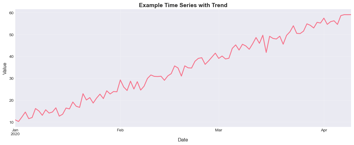
Sample size: 100
Mean: 34.54
Standard deviation: 14.70
2. Stationarity
2.1 Strong (Strict) Stationarity
A time series is strictly stationary if the joint distribution of is the same as that of for all and all lags .
Implication: The statistical properties are invariant to shifts in time.
2.2 Weak (Covariance) Stationarity
A time series is weakly stationary (or covariance stationary) if:
Constant mean: for all
Constant variance: for all
Autocovariance depends only on lag: for all and lag
2.3 Why Stationarity Matters
Most time series models (ARIMA, GARCH, VAR) assume stationarity
Non-stationary series can lead to spurious regression
Forecasting with non-stationary data is problematic
Many statistical properties (ergodicity, law of large numbers) require stationarity
2.4 Common Violations of Stationarity
Trend-stationary:
Difference-stationary: (random walk)
Structural breaks: Parameters change at specific points in time
Heteroskedasticity: Variance changes over time
Source
# Generate different types of processes
T = 500
t = np.arange(T)

# 1. Stationary process (AR(1) with |φ| < 1)
phi = 0.7
stationary = np.zeros(T)
epsilon = np.random.normal(0, 1, T)
for i in range(1, T):
    stationary[i] = phi * stationary[i-1] + epsilon[i]

# 2. Trend-stationary process
trend_stationary = 10 + 0.05 * t + np.random.normal(0, 1, T)

# 3. Difference-stationary (random walk)
random_walk = np.cumsum(np.random.normal(0, 1, T))

# 4. Random walk with drift
random_walk_drift = np.cumsum(np.random.normal(0.1, 1, T))

# Plot all processes
fig, axes = plt.subplots(2, 2, figsize=(15, 10))

axes[0, 0].plot(stationary, linewidth=1.5)
axes[0, 0].set_title('Stationary Process (AR(1))', fontsize=12, fontweight='bold')
axes[0, 0].axhline(y=0, color='r', linestyle='--', alpha=0.5)
axes[0, 0].grid(True, alpha=0.3)

axes[0, 1].plot(trend_stationary, linewidth=1.5)
axes[0, 1].set_title('Trend-Stationary Process', fontsize=12, fontweight='bold')
axes[0, 1].grid(True, alpha=0.3)

axes[1, 0].plot(random_walk, linewidth=1.5)
axes[1, 0].set_title('Random Walk (Difference-Stationary)', fontsize=12, fontweight='bold')
axes[1, 0].axhline(y=0, color='r', linestyle='--', alpha=0.5)
axes[1, 0].grid(True, alpha=0.3)

axes[1, 1].plot(random_walk_drift, linewidth=1.5)
axes[1, 1].set_title('Random Walk with Drift', fontsize=12, fontweight='bold')
axes[1, 1].grid(True, alpha=0.3)

for ax in axes.flat:
    ax.set_xlabel('Time', fontsize=10)
    ax.set_ylabel('Value', fontsize=10)

plt.tight_layout()
plt.show()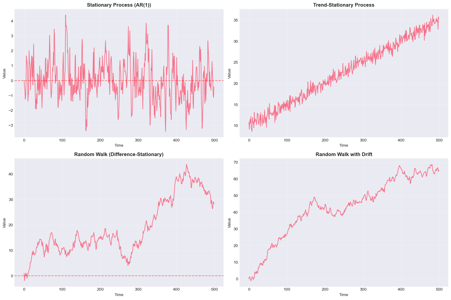
3. Testing for Stationarity
3.1 Augmented Dickey-Fuller (ADF) Test
The ADF test checks for the presence of a unit root:
Hypotheses:
: (unit root exists, series is non-stationary)
: (no unit root, series is stationary)
Decision rule: If p-value < 0.05, reject and conclude the series is stationary.
3.2 KPSS Test
The KPSS (Kwiatkowski-Phillips-Schmidt-Shin) test has opposite hypotheses:
Hypotheses:
: Series is stationary
: Series has a unit root
Decision rule: If p-value < 0.05, reject and conclude the series is non-stationary.
3.3 Combining Tests
Best practice: Use both tests for robustness
| ADF Result | KPSS Result | Conclusion |
|---|---|---|
| Stationary | Stationary | Stationary |
| Non-stationary | Non-stationary | Non-stationary |
| Stationary | Non-stationary | Trend-stationary |
| Non-stationary | Stationary | Difference-stationary |
Source
def test_stationarity(timeseries, name='Series', verbose=True):
    """
    Perform ADF and KPSS tests for stationarity.

    Parameters:
    -----------
    timeseries : array-like
        The time series to test
    name : str
        Name of the series for display
    verbose : bool
        Whether to print detailed results

    Returns:
    --------
    dict : Dictionary containing test results
    """

    # ADF Test
    adf_result = adfuller(timeseries, autolag='AIC')
    adf_statistic = adf_result[0]
    adf_pvalue = adf_result[1]
    adf_lags = adf_result[2]
    adf_critical_values = adf_result[4]

    # KPSS Test
    kpss_result = kpss(timeseries, regression='ct', nlags='auto')
    kpss_statistic = kpss_result[0]
    kpss_pvalue = kpss_result[1]
    kpss_lags = kpss_result[2]
    kpss_critical_values = kpss_result[3]

    if verbose:
        print(f"\n{'='*60}")
        print(f"Stationarity Tests for: {name}")
        print(f"{'='*60}")

        print("\n1. Augmented Dickey-Fuller Test")
        print("-" * 40)
        print(f"Test Statistic: {adf_statistic:.4f}")
        print(f"P-value: {adf_pvalue:.4f}")
        print(f"Lags used: {adf_lags}")
        print("Critical Values:")
        for key, value in adf_critical_values.items():
            print(f"  {key}: {value:.4f}")

        if adf_pvalue < 0.05:
            print("\n✓ ADF: Reject H0 → Series is STATIONARY (at 5% level)")
        else:
            print("\n✗ ADF: Fail to reject H0 → Series is NON-STATIONARY")

        print("\n2. KPSS Test")
        print("-" * 40)
        print(f"Test Statistic: {kpss_statistic:.4f}")
        print(f"P-value: {kpss_pvalue:.4f}")
        print(f"Lags used: {kpss_lags}")
        print("Critical Values:")
        for key, value in kpss_critical_values.items():
            print(f"  {key}: {value:.4f}")

        if kpss_pvalue < 0.05:
            print("\n✗ KPSS: Reject H0 → Series is NON-STATIONARY (at 5% level)")
        else:
            print("\n✓ KPSS: Fail to reject H0 → Series is STATIONARY")

        print("\n" + "="*60)

    return {
        'adf_statistic': adf_statistic,
        'adf_pvalue': adf_pvalue,
        'adf_is_stationary': adf_pvalue < 0.05,
        'kpss_statistic': kpss_statistic,
        'kpss_pvalue': kpss_pvalue,
        'kpss_is_stationary': kpss_pvalue >= 0.05
    }

# Test our generated series
test_stationarity(stationary, name='Stationary AR(1)')
test_stationarity(random_walk, name='Random Walk')
============================================================
Stationarity Tests for: Stationary AR(1)
============================================================

1. Augmented Dickey-Fuller Test
----------------------------------------
Test Statistic: -9.7416
P-value: 0.0000
Lags used: 0
Critical Values:
  1%: -3.4435
  5%: -2.8673
  10%: -2.5699

✓ ADF: Reject H0 → Series is STATIONARY (at 5% level)

2. KPSS Test
----------------------------------------
Test Statistic: 0.0571
P-value: 0.1000
Lags used: 10
Critical Values:
  10%: 0.1190
  5%: 0.1460
  2.5%: 0.1760
  1%: 0.2160

✓ KPSS: Fail to reject H0 → Series is STATIONARY

============================================================

============================================================
Stationarity Tests for: Random Walk
============================================================

1. Augmented Dickey-Fuller Test
----------------------------------------
Test Statistic: -1.5175
P-value: 0.5248
Lags used: 0
Critical Values:
  1%: -3.4435
  5%: -2.8673
  10%: -2.5699

✗ ADF: Fail to reject H0 → Series is NON-STATIONARY

2. KPSS Test
----------------------------------------
Test Statistic: 0.5071
P-value: 0.0100
Lags used: 12
Critical Values:
  10%: 0.1190
  5%: 0.1460
  2.5%: 0.1760
  1%: 0.2160

✗ KPSS: Reject H0 → Series is NON-STATIONARY (at 5% level)

============================================================
{'adf_statistic': -1.5175165267153008,
 'adf_pvalue': 0.5248290551329203,
 'adf_is_stationary': False,
 'kpss_statistic': 0.5070872812632301,
 'kpss_pvalue': 0.01,
 'kpss_is_stationary': False}
4. White Noise and Random Walks
4.1 White Noise
A white noise process satisfies:
for all
for all
for all
Properties:
Stationary
Unpredictable (best forecast is zero)
Building block for more complex models
Strong white noise additionally assumes
4.2 Random Walk
A random walk is defined as:
where is white noise.
Solution:
Properties:
Non-stationary
(constant)
(increases with time)
First difference is stationary:
Random walk with drift:
where is the drift parameter.
Source
# Generate and analyze white noise
T = 500
white_noise = np.random.normal(0, 1, T)

# Generate multiple random walk paths
n_paths = 5
random_walks = np.zeros((T, n_paths))
for i in range(n_paths):
    random_walks[:, i] = np.cumsum(np.random.normal(0, 1, T))

# Plotting
fig, axes = plt.subplots(2, 2, figsize=(15, 10))

# White noise time series
axes[0, 0].plot(white_noise, linewidth=1, alpha=0.7)
axes[0, 0].axhline(y=0, color='r', linestyle='--', alpha=0.5)
axes[0, 0].set_title('White Noise Process', fontsize=12, fontweight='bold')
axes[0, 0].set_xlabel('Time')
axes[0, 0].set_ylabel('Value')
axes[0, 0].grid(True, alpha=0.3)

# White noise histogram
axes[0, 1].hist(white_noise, bins=30, density=True, alpha=0.7, edgecolor='black')
x = np.linspace(white_noise.min(), white_noise.max(), 100)
axes[0, 1].plot(x, stats.norm.pdf(x, 0, 1), 'r-', linewidth=2, label='N(0,1)')
axes[0, 1].set_title('White Noise Distribution', fontsize=12, fontweight='bold')
axes[0, 1].set_xlabel('Value')
axes[0, 1].set_ylabel('Density')
axes[0, 1].legend()
axes[0, 1].grid(True, alpha=0.3)

# Multiple random walk paths
for i in range(n_paths):
    axes[1, 0].plot(random_walks[:, i], linewidth=1.5, alpha=0.7, label=f'Path {i+1}')
axes[1, 0].axhline(y=0, color='k', linestyle='--', alpha=0.3)
axes[1, 0].set_title('Multiple Random Walk Paths', fontsize=12, fontweight='bold')
axes[1, 0].set_xlabel('Time')
axes[1, 0].set_ylabel('Value')
axes[1, 0].legend()
axes[1, 0].grid(True, alpha=0.3)

# Random walk first difference (should be white noise)
rw_diff = np.diff(random_walks[:, 0])
axes[1, 1].plot(rw_diff, linewidth=1, alpha=0.7)
axes[1, 1].axhline(y=0, color='r', linestyle='--', alpha=0.5)
axes[1, 1].set_title('First Difference of Random Walk', fontsize=12, fontweight='bold')
axes[1, 1].set_xlabel('Time')
axes[1, 1].set_ylabel('Δy')
axes[1, 1].grid(True, alpha=0.3)

plt.tight_layout()
plt.show()

# Statistical tests
print("\nWhite Noise Statistics:")
print(f"Mean: {white_noise.mean():.4f} (expected: 0)")
print(f"Std Dev: {white_noise.std():.4f} (expected: 1)")
print(f"Skewness: {stats.skew(white_noise):.4f} (expected: 0)")
print(f"Kurtosis: {stats.kurtosis(white_noise):.4f} (expected: 0)")

# Ljung-Box test for white noise
from statsmodels.stats.diagnostic import acorr_ljungbox
lb_result = acorr_ljungbox(white_noise, lags=[10], return_df=True)
print(f"\nLjung-Box Q(10): {lb_result['lb_stat'].values[0]:.4f}")
print(f"P-value: {lb_result['lb_pvalue'].values[0]:.4f}")
if lb_result['lb_pvalue'].values[0] > 0.05:
    print("✓ Cannot reject null: Data consistent with white noise")
else:
    print("✗ Reject null: Data shows significant autocorrelation")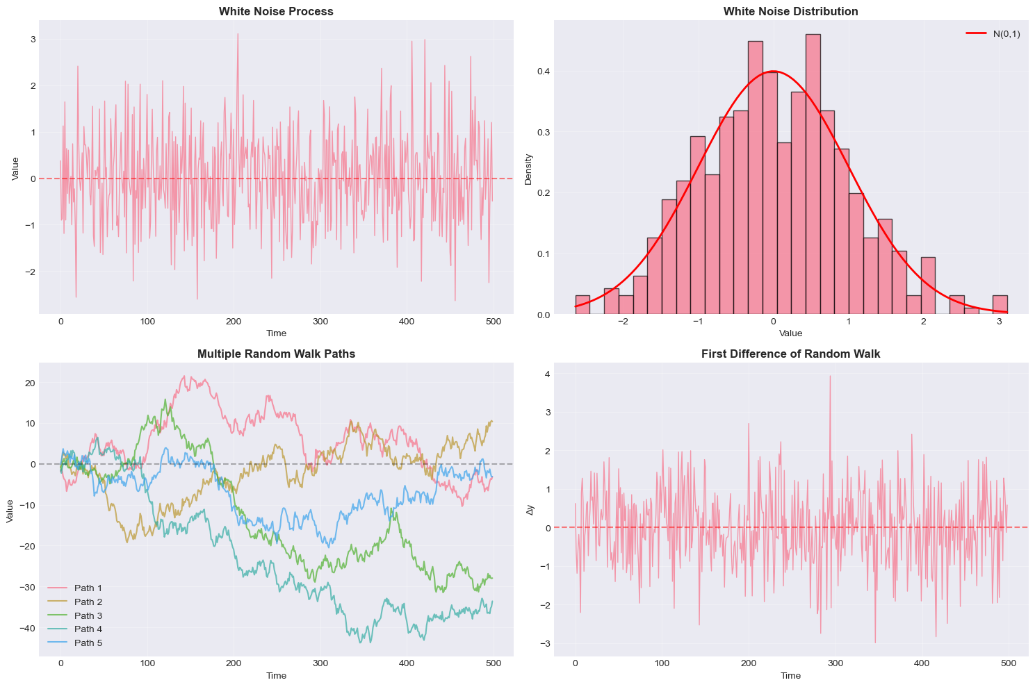
White Noise Statistics:
Mean: 0.0193 (expected: 0)
Std Dev: 0.9833 (expected: 1)
Skewness: 0.1279 (expected: 0)
Kurtosis: -0.0447 (expected: 0)

Ljung-Box Q(10): 18.7663
P-value: 0.0433
✗ Reject null: Data shows significant autocorrelation
5. Autocorrelation and Partial Autocorrelation
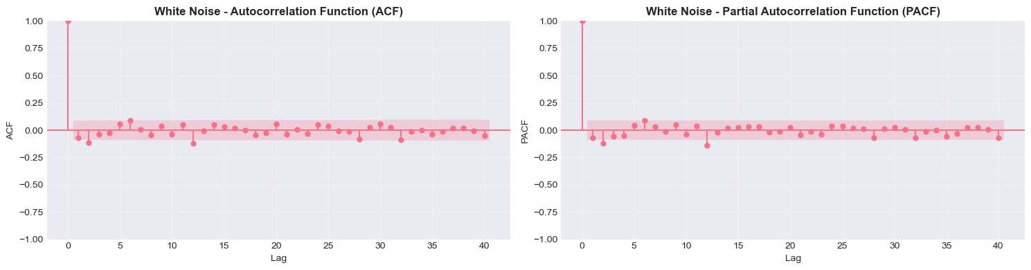
5.1 Autocorrelation Function (ACF)
The autocorrelation at lag measures the correlation between and :
Sample ACF:
Properties:
(correlation with itself)
For white noise: for all
Standard error (for white noise):
5.2 Partial Autocorrelation Function (PACF)
The partial autocorrelation at lag measures the correlation between and after removing the linear influence of .
It answers: “What is the direct correlation between and ?”
Mathematical definition: is the last coefficient in:
5.3 Interpreting ACF and PACF
| Process | ACF Pattern | PACF Pattern |
|---|---|---|
| White Noise | All zero | All zero |
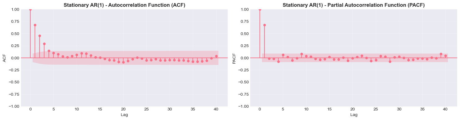
| AR(p) | Decays exponentially | Cuts off after lag p |
| MA(q) | Cuts off after lag q | Decays exponentially |
| ARMA(p,q) | Decays exponentially | Decays exponentially |
| Random Walk | Decays slowly | First lag ≈ 1 |
Source
def plot_acf_pacf(timeseries, lags=40, title=''):
    """
    Plot ACF and PACF for a time series.

    Parameters:
    -----------
    timeseries : array-like
        The time series to analyze
    lags : int
        Number of lags to display
    title : str
        Title prefix for the plots
    """
    fig, axes = plt.subplots(1, 2, figsize=(15, 4))

    # Plot ACF
    plot_acf(timeseries, lags=lags, ax=axes[0], alpha=0.05)
    axes[0].set_title(f'{title} - Autocorrelation Function (ACF)', fontsize=12, fontweight='bold')
    axes[0].set_xlabel('Lag', fontsize=10)
    axes[0].set_ylabel('ACF', fontsize=10)
    axes[0].grid(True, alpha=0.3)

    # Plot PACF
    plot_pacf(timeseries, lags=lags, ax=axes[1], alpha=0.05, method='ywm')
    axes[1].set_title(f'{title} - Partial Autocorrelation Function (PACF)', fontsize=12, fontweight='bold')
    axes[1].set_xlabel('Lag', fontsize=10)
    axes[1].set_ylabel('PACF', fontsize=10)
    axes[1].grid(True, alpha=0.3)

    plt.tight_layout()
    plt.show()

# Analyze white noise
print("White Noise Process")
plot_acf_pacf(white_noise, lags=40, title='White Noise')

# Analyze random walk
print("\nRandom Walk Process")
plot_acf_pacf(random_walks[:, 0], lags=40, title='Random Walk')

# Analyze stationary AR(1)
print("\nStationary AR(1) Process")
plot_acf_pacf(stationary, lags=40, title='Stationary AR(1)')
White Noise Process
Random Walk Process

Stationary AR(1) Process
Source
# Generate and compare different processes
T = 500

# AR(1) process: y_t = 0.8*y_{t-1} + ε_t
ar1 = np.zeros(T)
eps = np.random.normal(0, 1, T)
for i in range(1, T):
    ar1[i] = 0.8 * ar1[i-1] + eps[i]

# MA(1) process: y_t = ε_t + 0.8*ε_{t-1}
ma1 = np.zeros(T)
eps = np.random.normal(0, 1, T)
for i in range(1, T):
    ma1[i] = eps[i] + 0.8 * eps[i-1]

# Plot time series
fig, axes = plt.subplots(2, 2, figsize=(15, 8))

# AR(1) time series
axes[0, 0].plot(ar1, linewidth=1)
axes[0, 0].set_title('AR(1) Process: $y_t = 0.8y_{t-1} + \epsilon_t$', fontsize=11, fontweight='bold')
axes[0, 0].axhline(y=0, color='r', linestyle='--', alpha=0.5)
axes[0, 0].grid(True, alpha=0.3)

# MA(1) time series
axes[0, 1].plot(ma1, linewidth=1)
axes[0, 1].set_title('MA(1) Process: $y_t = \epsilon_t + 0.8\epsilon_{t-1}$', fontsize=11, fontweight='bold')
axes[0, 1].axhline(y=0, color='r', linestyle='--', alpha=0.5)
axes[0, 1].grid(True, alpha=0.3)

# AR(1) ACF and PACF combined
acf_ar = acf(ar1, nlags=20)
pacf_ar = pacf(ar1, nlags=20, method='ywm')
x = np.arange(len(acf_ar))
axes[1, 0].bar(x - 0.2, acf_ar, width=0.4, label='ACF', alpha=0.7)
axes[1, 0].bar(x + 0.2, pacf_ar, width=0.4, label='PACF', alpha=0.7)
axes[1, 0].axhline(y=0, color='black', linewidth=0.8)
axes[1, 0].axhline(y=1.96/np.sqrt(T), color='blue', linestyle='--', linewidth=1, alpha=0.5)
axes[1, 0].axhline(y=-1.96/np.sqrt(T), color='blue', linestyle='--', linewidth=1, alpha=0.5)
axes[1, 0].set_title('AR(1): ACF decays, PACF cuts off at lag 1', fontsize=11, fontweight='bold')
axes[1, 0].set_xlabel('Lag')
axes[1, 0].legend()
axes[1, 0].grid(True, alpha=0.3)

# MA(1) ACF and PACF combined
acf_ma = acf(ma1, nlags=20)
pacf_ma = pacf(ma1, nlags=20, method='ywm')
axes[1, 1].bar(x - 0.2, acf_ma, width=0.4, label='ACF', alpha=0.7)
axes[1, 1].bar(x + 0.2, pacf_ma, width=0.4, label='PACF', alpha=0.7)
axes[1, 1].axhline(y=0, color='black', linewidth=0.8)
axes[1, 1].axhline(y=1.96/np.sqrt(T), color='blue', linestyle='--', linewidth=1, alpha=0.5)
axes[1, 1].axhline(y=-1.96/np.sqrt(T), color='blue', linestyle='--', linewidth=1, alpha=0.5)
axes[1, 1].set_title('MA(1): ACF cuts off at lag 1, PACF decays', fontsize=11, fontweight='bold')
axes[1, 1].set_xlabel('Lag')
axes[1, 1].legend()
axes[1, 1].grid(True, alpha=0.3)

plt.tight_layout()
plt.show()

print("\nKey Observations:")
print("• AR(1): ACF decays exponentially, PACF has significant spike only at lag 1")
print("• MA(1): ACF has significant spike only at lag 1, PACF decays exponentially")
print("• Blue dashed lines show 95% confidence bands (±1.96/√T)")
Key Observations:
• AR(1): ACF decays exponentially, PACF has significant spike only at lag 1
• MA(1): ACF has significant spike only at lag 1, PACF decays exponentially
• Blue dashed lines show 95% confidence bands (±1.96/√T)
6. Practical Application: Real Financial Data
Let’s apply these concepts to real financial time series data.
Source
# Download financial data
print("Downloading financial data...")

# Download S&P 500 and Bitcoin data
tickers = ['^GSPC', 'BTC-USD', '^TNX']  # S&P 500, Bitcoin, 10-Year Treasury
data = yf.download(tickers, start='2020-01-01', end='2024-01-01', progress=False)

# Extract adjusted close prices
prices = data['Close']
prices.columns = ['SP500', 'BTC', 'TNX']
prices = prices.dropna()

# Calculate returns
returns = np.log(prices / prices.shift(1)).dropna() * 100  # Log returns in percentage

print(f"\nData period: {prices.index[0].date()} to {prices.index[-1].date()}")
print(f"Number of observations: {len(prices)}")
print(f"\nAssets: {', '.join(prices.columns)}")
Downloading financial data...
Data period: 2020-01-02 to 2023-12-29
Number of observations: 1006
Assets: SP500, BTC, TNX
Source
# Visualize price levels and returns
fig, axes = plt.subplots(3, 2, figsize=(15, 12))

assets = ['SP500', 'BTC', 'TNX']
titles = ['S&P 500', 'Bitcoin', '10-Year Treasury Yield']

for i, (asset, title) in enumerate(zip(assets, titles)):
    # Price levels
    axes[i, 0].plot(prices.index, prices[asset], linewidth=1.5)
    axes[i, 0].set_title(f'{title} - Price Level', fontsize=11, fontweight='bold')
    axes[i, 0].set_xlabel('Date')
    axes[i, 0].set_ylabel('Price')
    axes[i, 0].grid(True, alpha=0.3)

    # Returns
    axes[i, 1].plot(returns.index, returns[asset], linewidth=0.8, alpha=0.7)
    axes[i, 1].axhline(y=0, color='r', linestyle='--', alpha=0.5)
    axes[i, 1].set_title(f'{title} - Log Returns (%)', fontsize=11, fontweight='bold')
    axes[i, 1].set_xlabel('Date')
    axes[i, 1].set_ylabel('Return (%)')
    axes[i, 1].grid(True, alpha=0.3)

plt.tight_layout()
plt.show()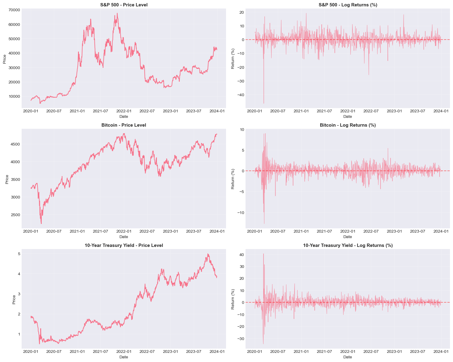
Source
# Descriptive statistics
print("\n" + "="*80)
print("DESCRIPTIVE STATISTICS")
print("="*80)

for asset in assets:
    print(f"\n{asset}:")
    print("-" * 60)

    ret = returns[asset].dropna()

    print(f"Returns:")
    print(f"  Mean: {ret.mean():.4f}%")
    print(f"  Std Dev: {ret.std():.4f}%")
    print(f"  Min: {ret.min():.4f}%")
    print(f"  Max: {ret.max():.4f}%")
    print(f"  Skewness: {stats.skew(ret):.4f}")
    print(f"  Kurtosis: {stats.kurtosis(ret):.4f}")

    # Jarque-Bera test for normality
    jb_stat, jb_pval = stats.jarque_bera(ret)
    print(f"\n  Jarque-Bera test (H0: Normal distribution):")
    print(f"    Statistic: {jb_stat:.4f}")
    print(f"    P-value: {jb_pval:.6f}")
    if jb_pval < 0.05:
        print(f"    ✗ Reject normality (at 5% level)")
    else:
        print(f"    ✓ Cannot reject normality")
================================================================================
DESCRIPTIVE STATISTICS
================================================================================

SP500:
------------------------------------------------------------
Returns:
  Mean: 0.1787%
  Std Dev: 4.2935%
  Min: -46.4730%
  Max: 19.1527%
  Skewness: -1.4686
  Kurtosis: 16.5810

  Jarque-Bera test (H0: Normal distribution):
    Statistic: 11873.8520
    P-value: 0.000000
    ✗ Reject normality (at 5% level)

BTC:
------------------------------------------------------------
Returns:
  Mean: 0.0379%
  Std Dev: 1.4561%
  Min: -12.7652%
  Max: 8.9683%
  Skewness: -0.7816
  Kurtosis: 12.7312

  Jarque-Bera test (H0: Normal distribution):
    Statistic: 6889.5927
    P-value: 0.000000
    ✗ Reject normality (at 5% level)

TNX:
------------------------------------------------------------
Returns:
  Mean: 0.0716%
  Std Dev: 4.2557%
  Min: -34.7009%
  Max: 40.4797%
  Skewness: 0.2095
  Kurtosis: 20.0543

  Jarque-Bera test (H0: Normal distribution):
    Statistic: 16848.4709
    P-value: 0.000000
    ✗ Reject normality (at 5% level)
Source
# Test stationarity for prices and returns
print("\n" + "="*80)
print("STATIONARITY TESTS")
print("="*80)

for asset in assets:
    print(f"\n{'='*80}")
    print(f"Asset: {asset}")
    print(f"{'='*80}")

    # Test price levels
    print("\n[PRICE LEVELS]")
    test_stationarity(prices[asset].dropna(), name=f'{asset} Prices', verbose=True)

    # Test returns
    print("\n[RETURNS]")
    test_stationarity(returns[asset].dropna(), name=f'{asset} Returns', verbose=True)
================================================================================
STATIONARITY TESTS
================================================================================

================================================================================
Asset: SP500
================================================================================

[PRICE LEVELS]

============================================================
Stationarity Tests for: SP500 Prices
============================================================

1. Augmented Dickey-Fuller Test
----------------------------------------
Test Statistic: -2.0154
P-value: 0.2798
Lags used: 22
Critical Values:
  1%: -3.4370
  5%: -2.8645
  10%: -2.5683

✗ ADF: Fail to reject H0 → Series is NON-STATIONARY

2. KPSS Test
----------------------------------------
Test Statistic: 0.7671
P-value: 0.0100
Lags used: 19
Critical Values:
  10%: 0.1190
  5%: 0.1460
  2.5%: 0.1760
  1%: 0.2160

✗ KPSS: Reject H0 → Series is NON-STATIONARY (at 5% level)

============================================================

[RETURNS]

============================================================
Stationarity Tests for: SP500 Returns
============================================================

1. Augmented Dickey-Fuller Test
----------------------------------------
Test Statistic: -11.1580
P-value: 0.0000
Lags used: 6
Critical Values:
  1%: -3.4369
  5%: -2.8644
  10%: -2.5683

✓ ADF: Reject H0 → Series is STATIONARY (at 5% level)

2. KPSS Test
----------------------------------------
Test Statistic: 0.1447
P-value: 0.0524
Lags used: 6
Critical Values:
  10%: 0.1190
  5%: 0.1460
  2.5%: 0.1760
  1%: 0.2160

✓ KPSS: Fail to reject H0 → Series is STATIONARY

============================================================

================================================================================
Asset: BTC
================================================================================

[PRICE LEVELS]

============================================================
Stationarity Tests for: BTC Prices
============================================================

1. Augmented Dickey-Fuller Test
----------------------------------------
Test Statistic: -1.4068
P-value: 0.5790
Lags used: 9
Critical Values:
  1%: -3.4369
  5%: -2.8644
  10%: -2.5683

✗ ADF: Fail to reject H0 → Series is NON-STATIONARY

2. KPSS Test
----------------------------------------
Test Statistic: 0.8059
P-value: 0.0100
Lags used: 19
Critical Values:
  10%: 0.1190
  5%: 0.1460
  2.5%: 0.1760
  1%: 0.2160

✗ KPSS: Reject H0 → Series is NON-STATIONARY (at 5% level)

============================================================

[RETURNS]

============================================================
Stationarity Tests for: BTC Returns
============================================================

1. Augmented Dickey-Fuller Test
----------------------------------------
Test Statistic: -9.3706
P-value: 0.0000
Lags used: 8
Critical Values:
  1%: -3.4369
  5%: -2.8644
  10%: -2.5683

✓ ADF: Reject H0 → Series is STATIONARY (at 5% level)

2. KPSS Test
----------------------------------------
Test Statistic: 0.0644
P-value: 0.1000
Lags used: 9
Critical Values:
  10%: 0.1190
  5%: 0.1460
  2.5%: 0.1760
  1%: 0.2160

✓ KPSS: Fail to reject H0 → Series is STATIONARY

============================================================

================================================================================
Asset: TNX
================================================================================

[PRICE LEVELS]

============================================================
Stationarity Tests for: TNX Prices
============================================================

1. Augmented Dickey-Fuller Test
----------------------------------------
Test Statistic: -0.2905
P-value: 0.9268
Lags used: 2
Critical Values:
  1%: -3.4369
  5%: -2.8644
  10%: -2.5683

✗ ADF: Fail to reject H0 → Series is NON-STATIONARY

2. KPSS Test
----------------------------------------
Test Statistic: 0.5141
P-value: 0.0100
Lags used: 19
Critical Values:
  10%: 0.1190
  5%: 0.1460
  2.5%: 0.1760
  1%: 0.2160

✗ KPSS: Reject H0 → Series is NON-STATIONARY (at 5% level)

============================================================

[RETURNS]

============================================================
Stationarity Tests for: TNX Returns
============================================================

1. Augmented Dickey-Fuller Test
----------------------------------------
Test Statistic: -5.7259
P-value: 0.0000
Lags used: 22
Critical Values:
  1%: -3.4370
  5%: -2.8645
  10%: -2.5683

✓ ADF: Reject H0 → Series is STATIONARY (at 5% level)

2. KPSS Test
----------------------------------------
Test Statistic: 0.1848
P-value: 0.0217
Lags used: 27
Critical Values:
  10%: 0.1190
  5%: 0.1460
  2.5%: 0.1760
  1%: 0.2160

✗ KPSS: Reject H0 → Series is NON-STATIONARY (at 5% level)

============================================================
Source
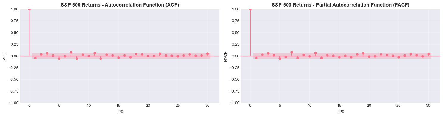
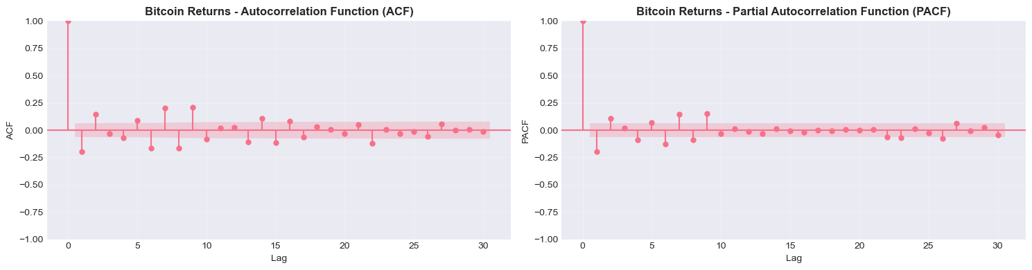
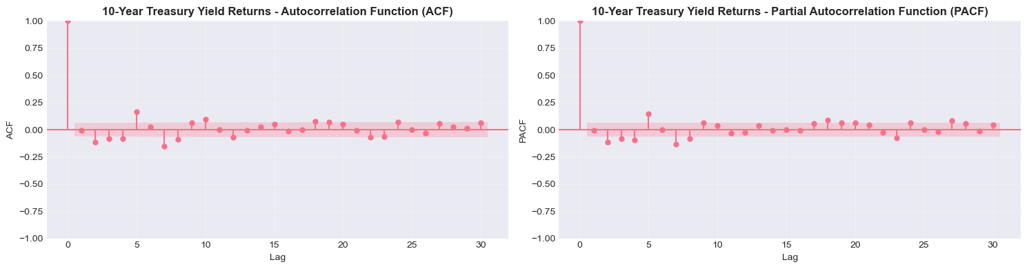
# ACF and PACF for returns
print("\nAutocorrelation Analysis of Returns")
print("="*80)

for asset, title in zip(assets, titles):
    print(f"\n{title}")
    plot_acf_pacf(returns[asset].dropna(), lags=30, title=f'{title} Returns')
Autocorrelation Analysis of Returns
================================================================================

S&P 500
Bitcoin
10-Year Treasury Yield
Source
# Test for autocorrelation in returns and squared returns
from statsmodels.stats.diagnostic import acorr_ljungbox

print("\nLjung-Box Tests for Autocorrelation")
print("="*80)

for asset, title in zip(assets, titles):
    print(f"\n{title}:")
    print("-" * 60)

    ret = returns[asset].dropna()
    ret_sq = ret ** 2

    # Test returns
    lb_ret = acorr_ljungbox(ret, lags=[10, 20], return_df=True)
    print("\nReturns:")
    print(lb_ret.to_string())

    # Test squared returns (proxy for volatility clustering)
    lb_sq = acorr_ljungbox(ret_sq, lags=[10, 20], return_df=True)
    print("\nSquared Returns (volatility):")
    print(lb_sq.to_string())

    if lb_sq['lb_pvalue'].iloc[-1] < 0.05:
        print("\n✓ Evidence of volatility clustering (GARCH effects likely)")
    else:
        print("\n✗ No strong evidence of volatility clustering")
Ljung-Box Tests for Autocorrelation
================================================================================

S&P 500:
------------------------------------------------------------

Returns:
      lb_stat  lb_pvalue
10  20.309707   0.026456
20  34.351273   0.023844

Squared Returns (volatility):
      lb_stat  lb_pvalue
10  21.246715   0.019437
20  22.952011   0.291157

✗ No strong evidence of volatility clustering

Bitcoin:
------------------------------------------------------------

Returns:
       lb_stat     lb_pvalue
10  223.211167  2.272727e-42
20  275.466384  8.015588e-47

Squared Returns (volatility):
        lb_stat      lb_pvalue
10  1286.284029  3.488940e-270
20  1471.811471  4.437857e-300

✓ Evidence of volatility clustering (GARCH effects likely)

10-Year Treasury Yield:
------------------------------------------------------------

Returns:
       lb_stat     lb_pvalue
10   99.660254  6.373216e-17
20  121.400995  1.568106e-16

Squared Returns (volatility):
        lb_stat      lb_pvalue
10  1173.519933  7.412772e-246
20  1222.565773  1.111894e-246

✓ Evidence of volatility clustering (GARCH effects likely)
7. Key Takeaways and Summary
Concepts Covered:
Time Series Fundamentals
Time series are ordered sequences where temporal dependence matters
Key features: trends, seasonality, cycles, and irregular components
Stationarity
Weak stationarity requires constant mean, variance, and autocovariance
Most time series models assume stationarity
Non-stationary series can often be made stationary through differencing or detrending
Testing for Stationarity
ADF test: H₀ is unit root (non-stationary)
KPSS test: H₀ is stationarity
Use both tests for robustness
White Noise and Random Walks
White noise is stationary and unpredictable
Random walks are non-stationary with variance growing over time
First differencing transforms random walks to white noise
Autocorrelation Analysis
ACF measures total correlation at each lag
PACF measures direct correlation after removing intermediate effects
ACF/PACF patterns help identify appropriate models
Financial Data Characteristics
Price levels are typically non-stationary
Returns are typically stationary but may show autocorrelation
Squared returns often show strong autocorrelation (volatility clustering)
Returns are often non-normal (fat tails, skewness)
Next Session Preview:
In Session 2, we will cover:
Classical time series decomposition
Smoothing techniques (moving averages, exponential smoothing)
Trend extraction methods (Hodrick-Prescott filter)
Seasonal adjustment procedures
8. Exercises
Exercise 1: Simulation Study
Generate 1000 observations from the following processes and compare their ACF/PACF:
AR(2):
MA(2):
ARMA(1,1):
Exercise 2: Real Data Analysis
Download data for a different asset (e.g., EUR/USD exchange rate, crude oil prices) and:
Test price levels and returns for stationarity
Examine ACF and PACF
Test for volatility clustering
Compare findings with S&P 500 results
Exercise 3: Differencing
For a non-stationary series:
Apply first differencing and test for stationarity
If still non-stationary, apply second differencing
Determine the order of integration (I(0), I(1), or I(2))
Exercise 4: Seasonal Patterns
Download monthly economic data (e.g., retail sales, unemployment rate) and:
Plot the series and visually identify seasonal patterns
Calculate ACF and look for seasonal spikes
Discuss implications for modeling
Source
# Space for your solutions to exercises

# Exercise 1:
# Your code here

# Exercise 2:
# Your code here

# Exercise 3:
# Your code here

# Exercise 4:
# Your code here
References and Further Reading
Textbooks:
Hamilton, J.D. (1994). Time Series Analysis. Princeton University Press.
Tsay, R.S. (2010). Analysis of Financial Time Series (3rd ed.). Wiley.
Brockwell, P.J., & Davis, R.A. (2016). Introduction to Time Series and Forecasting (3rd ed.). Springer.
Lütkepohl, H. (2005). New Introduction to Multiple Time Series Analysis. Springer.
Papers:
Dickey, D.A., & Fuller, W.A. (1979). Distribution of the estimators for autoregressive time series with a unit root. Journal of the American Statistical Association, 74(366a), 427-431.
Kwiatkowski, D., Phillips, P.C., Schmidt, P., & Shin, Y. (1992). Testing the null hypothesis of stationarity against the alternative of a unit root. Journal of Econometrics, 54(1-3), 159-178.
Python Resources:
statsmodels documentation: https://
www .statsmodels .org/ Seabold, S., & Perktold, J. (2010). Statsmodels: Econometric and statistical modeling with Python. Proceedings of the 9th Python in Science Conference.
Instructor Contact: hhs.nl
Office Hours: [Mon-Fri 9am-5pm]