Lecture 8: Options - Open Modules

MIT 15.401 — Finance Theory I (Prof. Andrew Lo)¶

Readings: Brealey, Myers, and Allen — Chapters 20–21

Options are fundamentally different from forwards and futures. A forward contract obligates both sides to exchange. An option gives one side the right, but not the obligation, to trade. This asymmetry creates the characteristic nonlinear payoff that makes options so powerful — and so intellectually fascinating.

This session covers three big ideas:

Payoff diagrams and strategies — the visual language for understanding what options do, including protective puts, spreads, and straddles.
Put-call parity — a no-arbitrage relationship linking calls, puts, stocks, and bonds that requires no model at all.
The binomial option-pricing model (Cox, Ross, Rubinstein 1979) — a constructive proof that options can be priced by replication. The key insight: form a portfolio of stocks and bonds that exactly replicates the option payoff. The option must cost the same. The stunning implication: the probability of the stock going up or down doesn’t appear in the formula.

Table of Contents¶

# ============================================================
# Setup
# ============================================================
import numpy as np
import pandas as pd
import matplotlib.pyplot as plt
import matplotlib.ticker as mticker
from scipy.stats import norm
from scipy.optimize import brentq

plt.rcParams.update({
    'figure.figsize': (10, 5),
    'axes.spines.top': False,
    'axes.spines.right': False,
    'axes.grid': True,
    'grid.alpha': 0.3,
    'font.size': 12,
    'lines.linewidth': 2,
})

print("Libraries loaded successfully.")

Libraries loaded successfully.

1. Definitions and Terminology¶

Two Types of Options¶

	Call Option	Put Option
Right to	Buy the underlying at $K$	Sell the underlying at $K$
Valuable when	$S_T > K$ (price rises)	$S_T < K$ (price falls)
Payoff	$\max(S_T - K, 0)$	$\max(K - S_T, 0)$

Key Terms¶

Term	Definition
Underlying	The asset the option is written on (stock, index, commodity, etc.)
Strike price $K$	The price at which the option holder can buy/sell
Expiration date $T$	The date the option expires
Premium	The price paid to acquire the option
European	Can only be exercised at expiration
American	Can be exercised at any time up to expiration
In-the-money (ITM)	Call: $S > K$ ; Put: $S < K$ (positive intrinsic value)
At-the-money (ATM)	$S \approx K$
Out-of-the-money (OTM)	Call: $S < K$ ; Put: $S > K$ (zero intrinsic value)

Options as Insurance (Lo’s Slide 4)¶

A put option is fundamentally like an insurance policy: you pay a premium upfront, and if bad things happen (price drops below $K$ ), you’re protected. If nothing bad happens, you lose only the premium.

This is the key distinction from futures hedging (Session 7): futures eliminate both downside and upside. Options eliminate only the downside while preserving the upside — but you pay a premium for this asymmetry.

2. Option Payoffs at Expiration¶

Payoff Formulas¶

At expiration, the payoff depends only on the relationship between $S_T$ and $K$ :

Position	Payoff	Profit (net of premium)
Long call	$\max(S_T - K, 0)$	$\max(S_T - K, 0) - C$
Short call	$-\max(S_T - K, 0)$	$C - \max(S_T - K, 0)$
Long put	$\max(K - S_T, 0)$	$\max(K - S_T, 0) - P$
Short put	$-\max(K - S_T, 0)$	$P - \max(K - S_T, 0)$

Lo’s Payoff Table (Slide 9)¶

	$S_T < K$	$S_T = K$	$S_T > K$
Call payoff	0	0	$S_T - K$
Call profit	$-C$	$-C$	$S_T - K - C$
Put payoff	$K - S_T$	0	0
Put profit	$K - S_T - P$	$-P$	$-P$

# ============================================================
# Four Basic Option Positions — Lo's Slide 8
# ============================================================
K = 50
S = np.linspace(30, 70, 200)

# Premium assumptions for profit diagrams
C = 5   # call premium
P = 4   # put premium

fig, axes = plt.subplots(2, 2, figsize=(14, 10))
positions = [
    ('Long Call', np.maximum(S - K, 0), np.maximum(S - K, 0) - C, '#3498db'),
    ('Long Put', np.maximum(K - S, 0), np.maximum(K - S, 0) - P, '#e74c3c'),
    ('Short Call', -np.maximum(S - K, 0), C - np.maximum(S - K, 0), '#2ecc71'),
    ('Short Put', -np.maximum(K - S, 0), P - np.maximum(K - S, 0), '#e67e22'),
]

for ax, (title, payoff, profit, color) in zip(axes.flat, positions):
    ax.plot(S, payoff, color=color, linewidth=3, label='Payoff')
    ax.plot(S, profit, color=color, linewidth=2, linestyle='--', alpha=0.7, label='Profit')
    ax.axhline(y=0, color='#2c3e50', linewidth=1, alpha=0.5)
    ax.axvline(x=K, color='gray', linewidth=1, linestyle=':', alpha=0.4)
    ax.fill_between(S, 0, profit, where=profit > 0, alpha=0.1, color='#2ecc71')
    ax.fill_between(S, 0, profit, where=profit < 0, alpha=0.1, color='#e74c3c')
    ax.set_xlabel('Stock Price at Expiration ($S_T$)', fontsize=11)
    ax.set_ylabel('$ Payoff / Profit', fontsize=11)
    ax.set_title(title, fontsize=14, fontweight='bold')
    ax.legend(fontsize=10)
    ax.text(K + 0.5, ax.get_ylim()[0] + 1, f'K = ${K}', fontsize=9, color='gray')

plt.tight_layout()
plt.show()

print("Key observations:")
print("• Long call: unlimited upside, limited downside (lose at most the premium C)")
print("• Long put:  limited upside (max K-P when S→0), limited downside (lose P)")
print("• Short call: limited upside (earn C), UNLIMITED downside")
print("• Short put:  limited upside (earn P), large downside (lose up to K-P)")
print("\n• Long + Short payoffs sum to zero: options are zero-sum games")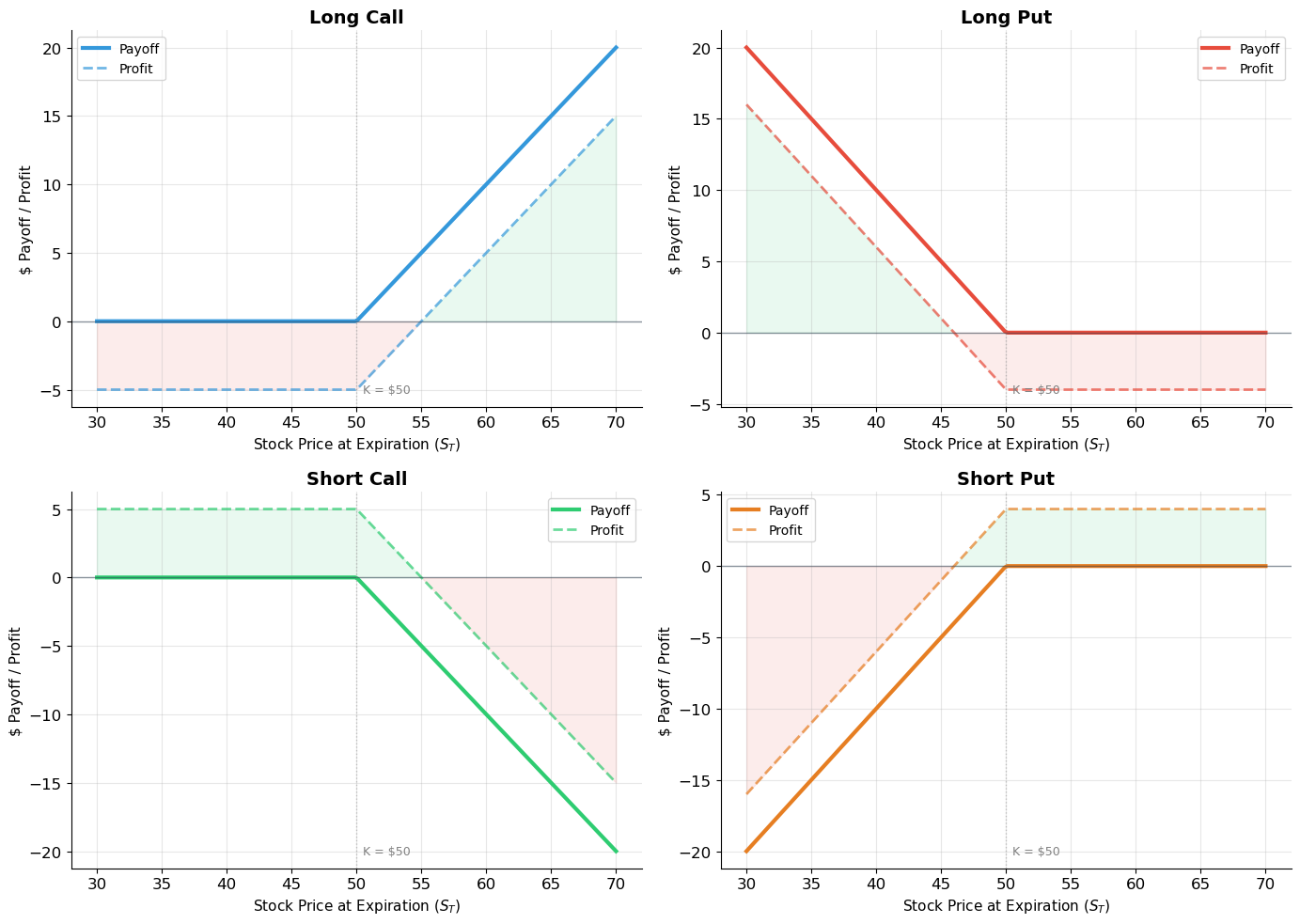

Key observations:
• Long call: unlimited upside, limited downside (lose at most the premium C)
• Long put:  limited upside (max K-P when S→0), limited downside (lose P)
• Short call: limited upside (earn C), UNLIMITED downside
• Short put:  limited upside (earn P), large downside (lose up to K-P)

• Long + Short payoffs sum to zero: options are zero-sum games

# ============================================================
# Leverage Effect: Stock Return vs. Call Option Return (Lo's Slide 6)
# ============================================================
# ▶ MODIFY AND RE-RUN
S0 = 50       # current stock price
K = 50        # strike price
C = 5         # call premium
# ============================================================

S_T = np.linspace(30, 70, 200)
stock_return = (S_T - S0) / S0 * 100
option_payoff = np.maximum(S_T - K, 0)
option_return = (option_payoff - C) / C * 100

fig, (ax1, ax2) = plt.subplots(1, 2, figsize=(14, 6))

# Left: Dollar payoffs
ax1.plot(S_T, S_T - S0, color='#2c3e50', linewidth=2.5, label='Stock P&L')
ax1.plot(S_T, option_payoff - C, color='#e74c3c', linewidth=2.5, label='Call P&L')
ax1.axhline(y=0, color='gray', linewidth=1, alpha=0.5)
ax1.axvline(x=K, color='gray', linewidth=1, linestyle=':', alpha=0.4)
ax1.set_xlabel('$S_T$', fontsize=12)
ax1.set_ylabel('Profit ($)', fontsize=12)
ax1.set_title('Dollar Profit: Stock vs. Call', fontsize=14, fontweight='bold')
ax1.legend(fontsize=11)

# Breakeven annotation
breakeven = K + C
ax1.annotate(f'Call breakeven\nS = ${breakeven}', xy=(breakeven, 0),
            xytext=(breakeven + 3, -8), fontsize=10, color='#e74c3c',
            arrowprops=dict(arrowstyle='->', color='#e74c3c'))

# Right: Percentage returns
ax2.plot(S_T, stock_return, color='#2c3e50', linewidth=2.5, label='Stock return')
ax2.plot(S_T, np.clip(option_return, -100, 300), color='#e74c3c', linewidth=2.5, label='Call return')
ax2.axhline(y=0, color='gray', linewidth=1, alpha=0.5)
ax2.set_xlabel('$S_T$', fontsize=12)
ax2.set_ylabel('Return (%)', fontsize=12)
ax2.set_title('Percentage Return: Stock vs. Call\n(Lo\'s Slide 6)', fontsize=14, fontweight='bold')
ax2.legend(fontsize=11)
ax2.set_ylim(-120, 300)

# Show leverage
ax2.annotate('Options amplify returns\n(leverage effect)', xy=(60, 200),
            fontsize=11, color='#e74c3c', fontweight='bold',
            bbox=dict(boxstyle='round', facecolor='#fdf2f2', alpha=0.9))

plt.tight_layout()
plt.show()

# Specific examples
for S_T_val in [40, 45, 50, 55, 60]:
    s_ret = (S_T_val - S0) / S0 * 100
    o_pf = max(S_T_val - K, 0)
    o_ret = (o_pf - C) / C * 100
    print(f"S_T = ${S_T_val}: Stock return = {s_ret:+.0f}%,  Call return = {o_ret:+.0f}%")

print("\nThe option magnifies gains AND losses — this is leverage in action.")
print(f"Investment: stock costs ${S0}, call costs only ${C} (leverage = {S0/C:.0f}×)")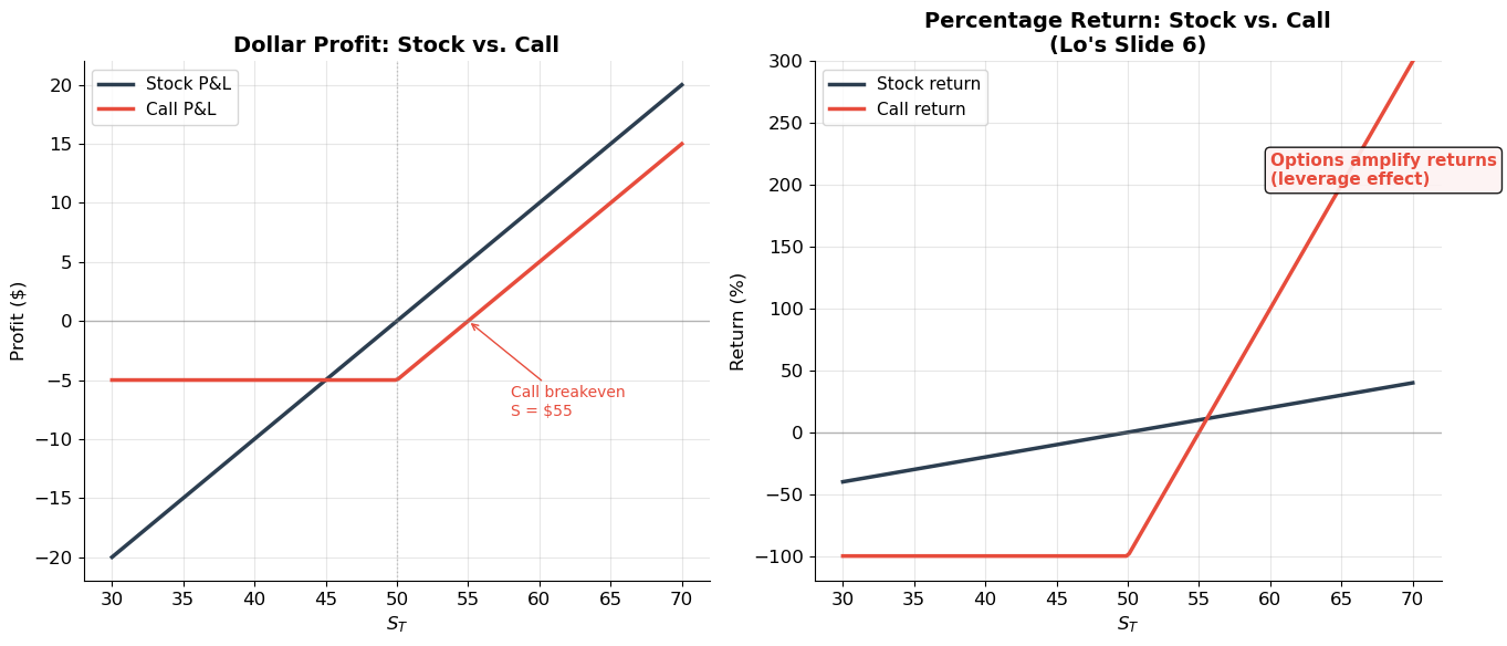

S_T = $40: Stock return = -20%,  Call return = -100%
S_T = $45: Stock return = -10%,  Call return = -100%
S_T = $50: Stock return = +0%,  Call return = -100%
S_T = $55: Stock return = +10%,  Call return = +0%
S_T = $60: Stock return = +20%,  Call return = +100%

The option magnifies gains AND losses — this is leverage in action.
Investment: stock costs $50, call costs only $5 (leverage = 10×)

3. Option Strategies¶

Options can be combined in various ways to create sophisticated payoff profiles. Lo presents three canonical strategies:

Strategy 1: Protective Put (Stock + Put)¶

Buy a stock AND buy a put with strike $K$ . This creates downside protection while preserving the upside — essentially portfolio insurance.

\text{Payoff} = S_T + \max(K - S_T, 0) = \max(S_T, K)

(1)

The portfolio can never be worth less than $K$ .

Strategy 2: Bull Call Spread (Buy Call₁, Sell Call₂)¶

Buy a call with low strike $K_1$ and sell a call with high strike $K_2 > K_1$ . This bets on a moderate price increase.

\text{Payoff} = \max(S_T - K_1, 0) - \max(S_T - K_2, 0)

(2)

Maximum payoff is $K_2 - K_1$ (capped upside), but the net premium is lower than buying a call alone.

Strategy 3: Straddle (Call + Put, same strike)¶

Buy a call AND a put with the same strike $K$ . This bets on volatility — you profit if the stock moves significantly in either direction.

\text{Payoff} = \max(S_T - K, 0) + \max(K - S_T, 0) = |S_T - K|

(3)

# ============================================================
# Lo's Three Option Strategies (Slides 11-13)
# ============================================================
K = 50
K1, K2 = 50, 60
S = np.linspace(30, 70, 200)

# Premiums
C_K = 5       # call at K=50
C_K2 = 2      # call at K=60
P_K = 4       # put at K=50

fig, axes = plt.subplots(2, 3, figsize=(18, 10))

# --- Strategy 1: Protective Put (Slide 11) ---
stock_payoff = S
put_payoff = np.maximum(K - S, 0)
protput_payoff = stock_payoff + put_payoff
protput_profit = protput_payoff - (50 + P_K)

# Top row: payoff components
axes[0, 0].plot(S, stock_payoff, color='#2c3e50', linewidth=2, label='Stock')
axes[0, 0].plot(S, put_payoff, color='#e74c3c', linewidth=2, linestyle='--', label='Put')
axes[0, 0].plot(S, protput_payoff, color='#3498db', linewidth=3, label='Stock + Put')
axes[0, 0].axhline(y=K, color='gray', linewidth=1, linestyle=':', alpha=0.5)
axes[0, 0].set_title('Protective Put — Payoff\n(Lo\'s Slide 11)', fontsize=13, fontweight='bold')
axes[0, 0].legend(fontsize=9)
axes[0, 0].set_ylabel('Payoff ($)', fontsize=11)
axes[0, 0].annotate(f'Floor at K = ${K}', xy=(35, K), fontsize=10, color='#3498db', fontweight='bold')

# --- Strategy 2: Bull Spread (Slide 12) ---
long_call = np.maximum(S - K1, 0)
short_call = -np.maximum(S - K2, 0)
spread_payoff = long_call + short_call
spread_profit = spread_payoff - (C_K - C_K2)

axes[0, 1].plot(S, long_call, color='#3498db', linewidth=2, linestyle='--', label=f'Long call K={K1}')
axes[0, 1].plot(S, short_call, color='#e74c3c', linewidth=2, linestyle='--', label=f'Short call K={K2}')
axes[0, 1].plot(S, spread_payoff, color='#2c3e50', linewidth=3, label='Bull Spread')
axes[0, 1].axhline(y=0, color='gray', linewidth=1, alpha=0.3)
axes[0, 1].set_title('Bull Call Spread — Payoff\n(Lo\'s Slide 12)', fontsize=13, fontweight='bold')
axes[0, 1].legend(fontsize=9)

# --- Strategy 3: Straddle (Slide 13) ---
call_K = np.maximum(S - K, 0)
put_K = np.maximum(K - S, 0)
straddle_payoff = call_K + put_K
straddle_profit = straddle_payoff - (C_K + P_K)

axes[0, 2].plot(S, call_K, color='#3498db', linewidth=2, linestyle='--', label='Call')
axes[0, 2].plot(S, put_K, color='#e74c3c', linewidth=2, linestyle='--', label='Put')
axes[0, 2].plot(S, straddle_payoff, color='#2c3e50', linewidth=3, label='Straddle')
axes[0, 2].axhline(y=0, color='gray', linewidth=1, alpha=0.3)
axes[0, 2].set_title('Straddle — Payoff\n(Lo\'s Slide 13)', fontsize=13, fontweight='bold')
axes[0, 2].legend(fontsize=9)

# Bottom row: profit diagrams
for ax, profit, title, cost_str in [
    (axes[1, 0], protput_profit, 'Protective Put', f'Stock + Put cost: ${50+P_K}'),
    (axes[1, 1], spread_profit, 'Bull Spread', f'Net premium: ${C_K - C_K2}'),
    (axes[1, 2], straddle_profit, 'Straddle', f'Total premium: ${C_K + P_K}'),
]:
    ax.plot(S, profit, color='#2c3e50', linewidth=3)
    ax.axhline(y=0, color='gray', linewidth=1, alpha=0.5)
    ax.fill_between(S, 0, profit, where=profit > 0, alpha=0.15, color='#2ecc71')
    ax.fill_between(S, 0, profit, where=profit < 0, alpha=0.15, color='#e74c3c')
    ax.set_title(f'{title} — Profit', fontsize=13, fontweight='bold')
    ax.set_xlabel('$S_T$', fontsize=11)
    ax.set_ylabel('Profit ($)', fontsize=11)
    ax.text(0.02, 0.95, cost_str, transform=ax.transAxes, fontsize=9, va='top',
            bbox=dict(boxstyle='round', facecolor='#f0f0f0', alpha=0.9))

plt.tight_layout()
plt.show()

print("Strategy insights:")
print("• Protective put: Insurance with a floor. You pay the put premium for downside protection.")
print("• Bull spread: Cheaper than a naked call, but capped upside. Good for moderate bullish views.")
print("• Straddle: A bet on VOLATILITY, not direction. Profits if the stock moves big in either direction.")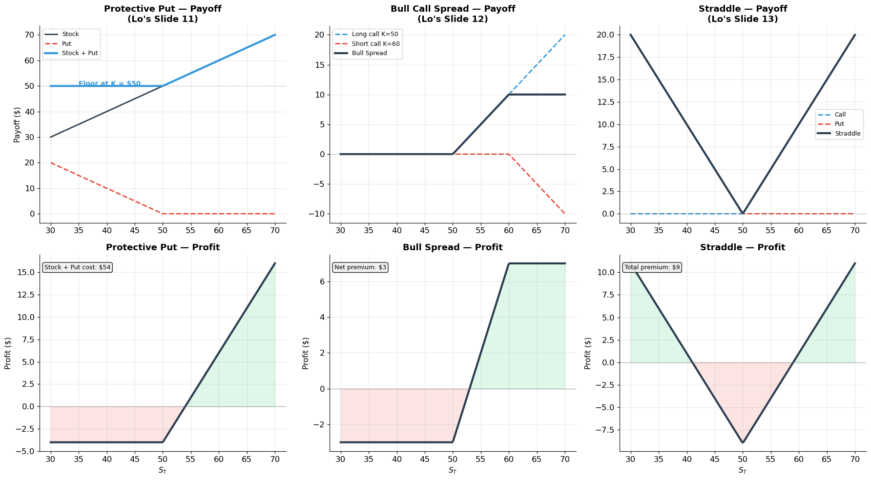

Strategy insights:
• Protective put: Insurance with a floor. You pay the put premium for downside protection.
• Bull spread: Cheaper than a naked call, but capped upside. Good for moderate bullish views.
• Straddle: A bet on VOLATILITY, not direction. Profits if the stock moves big in either direction.

4. Put-Call Parity¶

The Fundamental No-Arbitrage Relationship¶

Consider two portfolios:

Portfolio A: One call option with strike $K$ + Cash equal to $KB$ (= PV of $K$ )

Portfolio B: One put option with strike $K$ + One share of stock

At expiration:

State	Portfolio A	Portfolio B
$S_T < K$	$0 + K = K$	$(K - S_T) + S_T = K$
$S_T > K$	$(S_T - K) + K = S_T$	$0 + S_T = S_T$
$S_T = K$	$0 + K = K$	$0 + K = K$

Identical payoffs in every state! Therefore, by no-arbitrage:

\boxed{C + KB = P + S \quad \Longleftrightarrow \quad C - P = S - KB}

(4)

where $B = 1/(1+r)^T$ is the discount factor (price of a zero-coupon bond paying $1 at $T$ ).

This is put-call parity (for European options on non-dividend-paying stocks). It holds regardless of any model assumptions — it is a pure no-arbitrage result.

Implications¶

Knowing $C$ , $S$ , $K$ , and $r$ determines $P$ (and vice versa). You don’t need a pricing model!
Violations create arbitrage opportunities.
The relationship tells us: $\text{Call} - \text{Put} = \text{Stock} - \text{Bond}$ . A call is like a “leveraged stock position” and a put is like “insurance”.

# ============================================================
# Put-Call Parity: Visual Proof
# ============================================================
K = 50
S = np.linspace(30, 70, 200)
B = 1 / 1.05  # discount factor (5% rate)

fig, axes = plt.subplots(1, 3, figsize=(18, 5))

# Portfolio A: Call + Bond
call_payoff = np.maximum(S - K, 0)
bond_payoff = np.full_like(S, K)
portA = call_payoff + bond_payoff

axes[0].plot(S, call_payoff, color='#3498db', linewidth=2, linestyle='--', label='Call (K=50)')
axes[0].plot(S, bond_payoff, color='#e67e22', linewidth=2, linestyle=':', label=f'Bond (face={K})')
axes[0].plot(S, portA, color='#2c3e50', linewidth=3, label='Portfolio A')
axes[0].set_title('Portfolio A: Call + Bond', fontsize=14, fontweight='bold')
axes[0].legend(fontsize=10)
axes[0].set_xlabel('$S_T$', fontsize=12)
axes[0].set_ylabel('Payoff ($)', fontsize=12)

# Portfolio B: Put + Stock
put_payoff = np.maximum(K - S, 0)
stock_payoff = S
portB = put_payoff + stock_payoff

axes[1].plot(S, put_payoff, color='#e74c3c', linewidth=2, linestyle='--', label='Put (K=50)')
axes[1].plot(S, stock_payoff, color='#2ecc71', linewidth=2, linestyle=':', label='Stock')
axes[1].plot(S, portB, color='#2c3e50', linewidth=3, label='Portfolio B')
axes[1].set_title('Portfolio B: Put + Stock', fontsize=14, fontweight='bold')
axes[1].legend(fontsize=10)
axes[1].set_xlabel('$S_T$', fontsize=12)

# Overlay both
axes[2].plot(S, portA, color='#3498db', linewidth=3, label='A: Call + Bond')
axes[2].plot(S, portB, color='#e74c3c', linewidth=3, linestyle='--', label='B: Put + Stock')
axes[2].set_title('Identical Payoffs → Put-Call Parity', fontsize=14, fontweight='bold')
axes[2].legend(fontsize=12)
axes[2].set_xlabel('$S_T$', fontsize=12)

axes[2].annotate('C + K·B = P + S', xy=(50, 50), fontsize=14,
                fontweight='bold', color='#2c3e50',
                bbox=dict(boxstyle='round,pad=0.5', facecolor='#f0f0f0', alpha=0.9))

plt.tight_layout()
plt.show()

# Numerical example
S0 = 50; K = 50; r = 0.05; T = 0.5
B_val = 1 / (1 + r)**T
print("=" * 60)
print("PUT-CALL PARITY — Numerical Example")
print("=" * 60)
print(f"S₀ = ${S0}, K = ${K}, r = {r:.0%}, T = {T} years")
print(f"Discount factor B = 1/(1+r)^T = {B_val:.6f}")
print(f"K·B = ${K*B_val:.4f}")
print(f"\nPut-Call Parity: C + K·B = P + S")
print(f"                 C - P = S - K·B = ${S0} - ${K*B_val:.4f} = ${S0 - K*B_val:.4f}")
print(f"\nIf C = $4.00, then P = C - (S - KB) = $4.00 - ${S0 - K*B_val:.4f} = ${4.00 - (S0 - K*B_val):.4f}")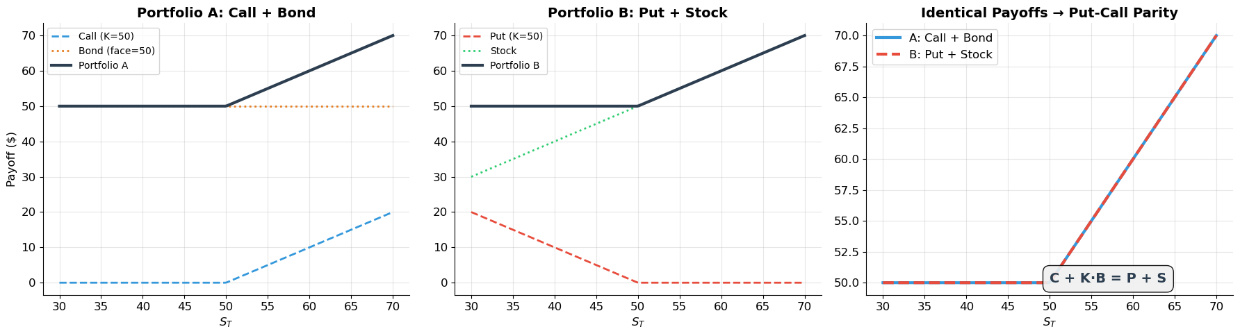

============================================================
PUT-CALL PARITY — Numerical Example
============================================================
S₀ = $50, K = $50, r = 5%, T = 0.5 years
Discount factor B = 1/(1+r)^T = 0.975900
K·B = $48.7950

Put-Call Parity: C + K·B = P + S
                 C - P = S - K·B = $50 - $48.7950 = $1.2050

If C = $4.00, then P = C - (S - KB) = $4.00 - $1.2050 = $2.7950

5. Determinants of Option Value¶

Six Key Factors¶

Factor	Effect on Call	Effect on Put	Intuition
Stock price $S$ ↑	↑	↓	Call more likely ITM; put less likely ITM
Strike price $K$ ↑	↓	↑	Higher hurdle for call; bigger floor for put
Time to expiration $T$ ↑	↑	↑	More time = more uncertainty = more option value
Volatility $\sigma$ ↑	↑	↑	More dispersion = higher expected payoff
Interest rate $r$ ↑	↑	↓	Lower PV of strike helps calls; hurts puts
Dividends $d$ ↑	↓	↑	Lower stock price at ex-date hurts calls

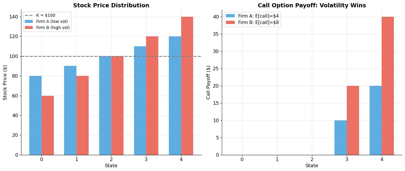
The Crucial Role of Volatility¶

Lo and the lecture notes both emphasize: option value increases with volatility. This is unique to options — for stocks and bonds, higher risk typically means a lower price (higher discount rate). For options, higher volatility increases the expected payoff because options have asymmetric payoffs: they benefit from extreme moves in one direction but are protected from the other.

# ============================================================
# Volatility and Option Value
# ============================================================
# Two stocks: same price, different volatility
S0 = 100; K = 100

# Firm A: low vol
states_A = [80, 90, 100, 110, 120]
probs = [0.1, 0.2, 0.4, 0.2, 0.1]

# Firm B: high vol
states_B = [60, 80, 100, 120, 140]

# Expected stock price (same)
E_A = sum(s * p for s, p in zip(states_A, probs))
E_B = sum(s * p for s, p in zip(states_B, probs))

# Expected call payoff (different!)
E_call_A = sum(max(s - K, 0) * p for s, p in zip(states_A, probs))
E_call_B = sum(max(s - K, 0) * p for s, p in zip(states_B, probs))

print("=" * 60)
print("VOLATILITY AND OPTION VALUE")
print("=" * 60)
print(f"Both stocks: current price = ${S0}, same expected value")
print(f"\n{'State':>8s} {'Prob':>6s} {'Firm A':>8s} {'A call':>8s} {'Firm B':>8s} {'B call':>8s}")
print("-" * 55)
for i in range(5):
    ca = max(states_A[i] - K, 0)
    cb = max(states_B[i] - K, 0)
    print(f"{i+1:>8d} {probs[i]:>6.1%} ${states_A[i]:>6d} ${ca:>6d} ${states_B[i]:>6d} ${cb:>6d}")

print(f"{'':>8s} {'':>6s} {'─'*8} {'─'*8} {'─'*8} {'─'*8}")
print(f"{'E[·]':>8s} {'':>6s} ${E_A:>6.0f} ${E_call_A:>6.0f} ${E_B:>6.0f} ${E_call_B:>6.0f}")
print(f"\nSame expected stock price: E[A] = E[B] = ${E_A:.0f}")
print(f"But E[call_B] = ${E_call_B:.0f} > E[call_A] = ${E_call_A:.0f}")
print(f"\n→ Higher volatility increases option value because the upside")
print(f"  is captured (S - K when S > K) but the downside is truncated (payoff = 0).")

# Visualization
fig, (ax1, ax2) = plt.subplots(1, 2, figsize=(14, 6))

x = np.arange(5)
width = 0.35
ax1.bar(x - width/2, states_A, width, color='#3498db', alpha=0.8, label='Firm A (low vol)')
ax1.bar(x + width/2, states_B, width, color='#e74c3c', alpha=0.8, label='Firm B (high vol)')
ax1.axhline(y=K, color='gray', linewidth=2, linestyle='--', label=f'K = ${K}')
ax1.set_xlabel('State', fontsize=12)
ax1.set_ylabel('Stock Price ($)', fontsize=12)
ax1.set_title('Stock Price Distribution', fontsize=14, fontweight='bold')
ax1.legend(fontsize=10)

call_A = [max(s - K, 0) for s in states_A]
call_B = [max(s - K, 0) for s in states_B]
ax2.bar(x - width/2, call_A, width, color='#3498db', alpha=0.8, label=f'Firm A: E[call]=${E_call_A:.0f}')
ax2.bar(x + width/2, call_B, width, color='#e74c3c', alpha=0.8, label=f'Firm B: E[call]=${E_call_B:.0f}')
ax2.set_xlabel('State', fontsize=12)
ax2.set_ylabel('Call Payoff ($)', fontsize=12)
ax2.set_title('Call Option Payoff: Volatility Wins', fontsize=14, fontweight='bold')
ax2.legend(fontsize=11)

plt.tight_layout()
plt.show()

============================================================
VOLATILITY AND OPTION VALUE
============================================================
Both stocks: current price = $100, same expected value

   State   Prob   Firm A   A call   Firm B   B call
-------------------------------------------------------
       1  10.0% $    80 $     0 $    60 $     0
       2  20.0% $    90 $     0 $    80 $     0
       3  40.0% $   100 $     0 $   100 $     0
       4  20.0% $   110 $    10 $   120 $    20
       5  10.0% $   120 $    20 $   140 $    40
                ──────── ──────── ──────── ────────
    E[·]        $   100 $     4 $   100 $     8

Same expected stock price: E[A] = E[B] = $100
But E[call_B] = $8 > E[call_A] = $4

→ Higher volatility increases option value because the upside
  is captured (S - K when S > K) but the downside is truncated (payoff = 0).

6. The Binomial Option-Pricing Model¶

The Setup (Lo’s Slides 16–21)¶

Consider a one-period model:

Current stock price: $S_0$
Tomorrow: stock goes up to $uS_0$ with probability $p$ , or down to $dS_0$ with probability $(1-p)$
Risk-free rate: $r$ (so $1 today becomes $r $tomorrow, where$ r = 1 + r_f$)
European call with strike $K$ , expiring tomorrow

\text{Call payoff: } C_u = \max(uS_0 - K, 0) \text{ or } C_d = \max(dS_0 - K, 0)

(5)

The Replicating Portfolio Argument¶

Key idea: Construct a portfolio of $\Delta$ shares of stock and $B in bonds that replicates the option payoff:

uS_0 \Delta + rB = C_u \quad \text{(up state)}

(6)

dS_0 \Delta + rB = C_d \quad \text{(down state)}

(7)

Solving these two equations:

\boxed{\Delta^* = \frac{C_u - C_d}{(u - d)S_0}} \qquad \boxed{B^* = \frac{uC_d - dC_u}{(u - d)r}}

(8)

Since this portfolio has identical payoffs to the option in every state, no-arbitrage requires:

\boxed{C_0 = S_0 \Delta^* + B^* = \frac{1}{r}\left[\frac{r - d}{u - d}C_u + \frac{u - r}{u - d}C_d\right]}

(9)

The Stunning Result¶

The probability $p$ does not appear anywhere in the formula!

Two investors who disagree completely about the probability of the stock going up must still agree on the option price. The option price is determined entirely by $S_0$ , $u$ , $d$ , $r$ , and $K$ — all observable quantities.

The terms $q = (r-d)/(u-d)$ and $(1-q) = (u-r)/(u-d)$ are called risk-neutral probabilities. They are not real probabilities — they are mathematical weights that arise from the replication argument.

# ============================================================
# One-Period Binomial Model — Detailed Derivation
# ============================================================

def binomial_one_period(S0, K, u, d, r):
    """One-period binomial option pricing.
    
    Returns: C0, delta, B, Cu, Cd, q
    r here is the GROSS risk-free rate (e.g. 1.10 for 10%).
    """
    Su = u * S0
    Sd = d * S0
    Cu = max(Su - K, 0)
    Cd = max(Sd - K, 0)
    
    delta = (Cu - Cd) / ((u - d) * S0)
    B = (u * Cd - d * Cu) / ((u - d) * r)
    C0 = S0 * delta + B
    
    # Risk-neutral probability
    q = (r - d) / (u - d)
    C0_check = (q * Cu + (1 - q) * Cd) / r
    
    return C0, delta, B, Cu, Cd, q


# Lecture notes example: S0=50, u=1.5, d=0.5, K=50, r=1.10
S0 = 50; K = 50; u = 1.5; d = 0.5; r = 1.10
C0, delta, B, Cu, Cd, q = binomial_one_period(S0, K, u, d, r)

print("=" * 70)
print("ONE-PERIOD BINOMIAL — Lecture Notes Example")
print("=" * 70)
print(f"S₀ = ${S0},  K = ${K},  u = {u},  d = {d},  r = {r}")
print(f"\nStock tree:")
print(f"  uS₀ = {u}×{S0} = ${u*S0:.0f}  (up state)")
print(f"  dS₀ = {d}×{S0} = ${d*S0:.0f}  (down state)")
print(f"\nCall payoffs:")
print(f"  Cᵤ = max({u*S0:.0f} - {K}, 0) = ${Cu:.2f}")
print(f"  C_d = max({d*S0:.0f} - {K}, 0) = ${Cd:.2f}")
print(f"\nReplicating portfolio:")
print(f"  Δ* = (Cᵤ - C_d)/((u-d)S₀) = ({Cu}-{Cd})/(({u}-{d})×{S0}) = {delta:.4f}")
print(f"  B* = (uC_d - dCᵤ)/((u-d)r) = ({u}×{Cd} - {d}×{Cu})/(({u}-{d})×{r}) = ${B:.4f}")
print(f"\nVerification:")
print(f"  Up state:   {delta:.4f}×{u*S0:.0f} + {r}×({B:.4f}) = {delta*u*S0 + r*B:.4f} = Cᵤ = {Cu:.2f} ✓")
print(f"  Down state: {delta:.4f}×{d*S0:.0f} + {r}×({B:.4f}) = {delta*d*S0 + r*B:.4f} = C_d = {Cd:.2f} ✓")
print(f"\nOption price:")
print(f"  C₀ = S₀Δ* + B* = {S0}×{delta:.4f} + ({B:.4f}) = ${C0:.4f}")
print(f"\nRisk-neutral probability:")
print(f"  q = (r-d)/(u-d) = ({r}-{d})/({u}-{d}) = {q:.4f}")
print(f"  C₀ = [q·Cᵤ + (1-q)·C_d]/r = [{q:.4f}×{Cu} + {1-q:.4f}×{Cd}]/{r} = ${(q*Cu+(1-q)*Cd)/r:.4f} ✓")
print(f"\nDelta (hedge ratio) = {delta:.4f}")
print(f"  → To hedge one call, hold {delta:.4f} shares and borrow ${-B:.2f}")

======================================================================
ONE-PERIOD BINOMIAL — Lecture Notes Example
======================================================================
S₀ = $50,  K = $50,  u = 1.5,  d = 0.5,  r = 1.1

Stock tree:
  uS₀ = 1.5×50 = $75  (up state)
  dS₀ = 0.5×50 = $25  (down state)

Call payoffs:
  Cᵤ = max(75 - 50, 0) = $25.00
  C_d = max(25 - 50, 0) = $0.00

Replicating portfolio:
  Δ* = (Cᵤ - C_d)/((u-d)S₀) = (25.0-0)/((1.5-0.5)×50) = 0.5000
  B* = (uC_d - dCᵤ)/((u-d)r) = (1.5×0 - 0.5×25.0)/((1.5-0.5)×1.1) = $-11.3636

Verification:
  Up state:   0.5000×75 + 1.1×(-11.3636) = 25.0000 = Cᵤ = 25.00 ✓
  Down state: 0.5000×25 + 1.1×(-11.3636) = 0.0000 = C_d = 0.00 ✓

Option price:
  C₀ = S₀Δ* + B* = 50×0.5000 + (-11.3636) = $13.6364

Risk-neutral probability:
  q = (r-d)/(u-d) = (1.1-0.5)/(1.5-0.5) = 0.6000
  C₀ = [q·Cᵤ + (1-q)·C_d]/r = [0.6000×25.0 + 0.4000×0]/1.1 = $13.6364 ✓

Delta (hedge ratio) = 0.5000
  → To hedge one call, hold 0.5000 shares and borrow $11.36

# ============================================================
# Two-Period Binomial Tree — Full Worked Example
# ============================================================

def binomial_tree(S0, K, u, d, r, n, option_type='call', american=False):
    """N-period binomial tree for European/American call or put.
    r is GROSS rate per period.
    Returns: price, stock_tree, option_tree, delta_tree
    """
    # Build stock tree
    stock = np.zeros((n + 1, n + 1))
    for i in range(n + 1):
        for j in range(i + 1):
            stock[j, i] = S0 * u**(i - j) * d**j
    
    # Option payoff at maturity
    opt = np.zeros((n + 1, n + 1))
    for j in range(n + 1):
        if option_type == 'call':
            opt[j, n] = max(stock[j, n] - K, 0)
        else:
            opt[j, n] = max(K - stock[j, n], 0)
    
    # Risk-neutral probability
    q = (r - d) / (u - d)
    
    # Backward induction
    delta = np.zeros((n, n))
    for i in range(n - 1, -1, -1):
        for j in range(i + 1):
            continuation = (q * opt[j, i + 1] + (1 - q) * opt[j + 1, i + 1]) / r
            if american:
                if option_type == 'call':
                    exercise = max(stock[j, i] - K, 0)
                else:
                    exercise = max(K - stock[j, i], 0)
                opt[j, i] = max(continuation, exercise)
            else:
                opt[j, i] = continuation
            # Delta at each node
            delta[j, i] = (opt[j, i+1] - opt[j+1, i+1]) / (stock[j, i+1] - stock[j+1, i+1])
    
    return opt[0, 0], stock, opt, delta


# Two-period example from lecture notes
S0 = 50; K = 50; u = 1.5; d = 0.5; r = 1.10; n = 2

C0, stock, opt, delta = binomial_tree(S0, K, u, d, r, n, 'call')

print("=" * 70)
print("TWO-PERIOD BINOMIAL TREE — Lecture Notes Example")
print(f"S₀ = ${S0}, K = ${K}, u = {u}, d = {d}, r = {r}, n = {n}")
print("=" * 70)

# Display stock tree
print("\nStock price tree:")
for j in range(n + 1):
    row = []
    for i in range(n + 1):
        if j <= i:
            row.append(f"${stock[j, i]:>7.2f}")
        else:
            row.append(f"{'':>8s}")
    print("  ".join(row))

print("\nOption value tree:")
for j in range(n + 1):
    row = []
    for i in range(n + 1):
        if j <= i:
            row.append(f"${opt[j, i]:>7.2f}")
        else:
            row.append(f"{'':>8s}")
    print("  ".join(row))

print(f"\nDelta (hedge ratio) tree:")
for j in range(n):
    row = []
    for i in range(n):
        if j <= i:
            row.append(f"{delta[j, i]:>7.4f}")
        else:
            row.append(f"{'':>8s}")
    print("  ".join(row))

print(f"\nCall price C₀ = ${C0:.4f}")
print(f"\nStep-by-step (matching lecture notes):")
print(f"  Period 2 payoffs: Cuu=${opt[0,2]:.2f}, Cud=${opt[1,2]:.2f}, Cdd=${opt[2,2]:.2f}")

# Verify Cu from period 1
q = (r - d) / (u - d)
Cu_check = (q * opt[0, 2] + (1 - q) * opt[1, 2]) / r
Cd_check = (q * opt[1, 2] + (1 - q) * opt[2, 2]) / r
print(f"  Period 1: Cu = (q×Cuu + (1-q)×Cud)/r = ({q:.3f}×{opt[0,2]:.2f} + {1-q:.3f}×{opt[1,2]:.2f})/{r} = ${Cu_check:.3f}")
print(f"            Cd = (q×Cud + (1-q)×Cdd)/r = ({q:.3f}×{opt[1,2]:.2f} + {1-q:.3f}×{opt[2,2]:.2f})/{r} = ${Cd_check:.3f}")
C0_check = (q * Cu_check + (1 - q) * Cd_check) / r
print(f"  Period 0: C0 = (q×Cu + (1-q)×Cd)/r = ({q:.3f}×{Cu_check:.3f} + {1-q:.3f}×{Cd_check:.3f})/{r} = ${C0_check:.3f}")
print(f"\n  Exercise value at period 1 up-node: ${u*S0 - K:.2f}")
print(f"  Continuation value:                 ${Cu_check:.3f}")
print(f"  No early exercise (Cu > exercise) ✓")

======================================================================
TWO-PERIOD BINOMIAL TREE — Lecture Notes Example
S₀ = $50, K = $50, u = 1.5, d = 0.5, r = 1.1, n = 2
======================================================================

Stock price tree:
$  50.00  $  75.00  $ 112.50
          $  25.00  $  37.50
                    $  12.50

Option value tree:
$  18.60  $  34.09  $  62.50
          $   0.00  $   0.00
                    $   0.00

Delta (hedge ratio) tree:
 0.6818   0.8333
           0.0000

Call price C₀ = $18.5950

Step-by-step (matching lecture notes):
  Period 2 payoffs: Cuu=$62.50, Cud=$0.00, Cdd=$0.00
  Period 1: Cu = (q×Cuu + (1-q)×Cud)/r = (0.600×62.50 + 0.400×0.00)/1.1 = $34.091
            Cd = (q×Cud + (1-q)×Cdd)/r = (0.600×0.00 + 0.400×0.00)/1.1 = $0.000
  Period 0: C0 = (q×Cu + (1-q)×Cd)/r = (0.600×34.091 + 0.400×0.000)/1.1 = $18.595

  Exercise value at period 1 up-node: $25.00
  Continuation value:                 $34.091
  No early exercise (Cu > exercise) ✓

# ============================================================
# Binomial Tree Visualization
# ============================================================

def draw_binomial_tree(stock, opt, delta, n, title, K):
    """Visualize the binomial tree."""
    fig, ax = plt.subplots(figsize=(max(12, 3*n), max(6, 2*n)))
    ax.set_xlim(-0.5, n + 0.5)
    y_vals = []
    for i in range(n + 1):
        for j in range(i + 1):
            y_vals.append(i - 2*j)
    y_min, y_max = min(y_vals) - 1, max(y_vals) + 1
    ax.set_ylim(y_min, y_max)
    ax.axis('off')
    ax.set_title(title, fontsize=16, fontweight='bold', pad=20)
    
    # Draw nodes and edges
    for i in range(n + 1):
        for j in range(i + 1):
            x = i
            y = i - 2 * j
            
            # Color based on option value
            if i == n:
                color = '#2ecc71' if opt[j, i] > 0 else '#e0e0e0'
            else:
                color = '#3498db'
            
            # Node
            txt = f"S={stock[j,i]:.0f}\nC={opt[j,i]:.2f}"
            if i < n:
                txt += f"\nΔ={delta[j,i]:.3f}"
            
            ax.annotate(txt, xy=(x, y), fontsize=8, ha='center', va='center',
                       bbox=dict(boxstyle='round,pad=0.4', facecolor=color, alpha=0.3, edgecolor='#2c3e50'))
            
            # Edges to next period
            if i < n:
                # Up
                x_next_u, y_next_u = i + 1, (i + 1) - 2 * j
                ax.annotate('', xy=(x_next_u - 0.15, y_next_u - 0.15), xytext=(x + 0.15, y + 0.15),
                           arrowprops=dict(arrowstyle='->', color='#2ecc71', lw=1.5))
                # Down
                x_next_d, y_next_d = i + 1, (i + 1) - 2 * (j + 1)
                ax.annotate('', xy=(x_next_d - 0.15, y_next_d + 0.15), xytext=(x + 0.15, y - 0.15),
                           arrowprops=dict(arrowstyle='->', color='#e74c3c', lw=1.5))
    
    # Period labels
    for i in range(n + 1):
        ax.text(i, y_max - 0.3, f't={i}', ha='center', fontsize=11, fontweight='bold', color='#2c3e50')
    
    plt.tight_layout()
    plt.show()


draw_binomial_tree(stock, opt, delta, n, f'Two-Period Binomial Tree (K=${K})', K)

print("Green nodes at maturity = in-the-money (positive payoff)")
print("Δ changes at each node — the replicating portfolio must be rebalanced dynamically")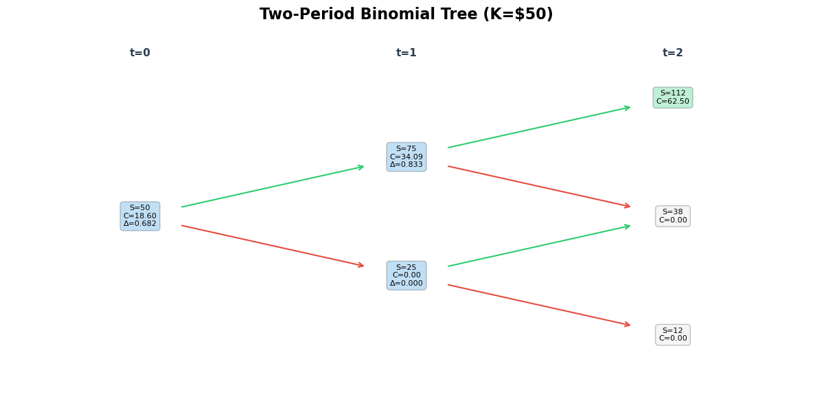

Green nodes at maturity = in-the-money (positive payoff)
Δ changes at each node — the replicating portfolio must be rebalanced dynamically

# ============================================================
# Multi-Period Convergence: Binomial → Black-Scholes
# ============================================================
# ▶ MODIFY AND RE-RUN
S0 = 50
K = 50
rf_annual = 0.05    # annual risk-free rate
sigma = 0.30        # annual volatility
T = 0.5             # 6 months
# ============================================================

# Black-Scholes price for comparison
def black_scholes_call(S, K, T, r, sigma):
    d1 = (np.log(S / K) + (r + sigma**2 / 2) * T) / (sigma * np.sqrt(T))
    d2 = d1 - sigma * np.sqrt(T)
    return S * norm.cdf(d1) - K * np.exp(-r * T) * norm.cdf(d2)

def black_scholes_put(S, K, T, r, sigma):
    d1 = (np.log(S / K) + (r + sigma**2 / 2) * T) / (sigma * np.sqrt(T))
    d2 = d1 - sigma * np.sqrt(T)
    return K * np.exp(-r * T) * norm.cdf(-d2) - S * norm.cdf(-d1)

BS_price = black_scholes_call(S0, K, T, rf_annual, sigma)

# Compute binomial prices for increasing n
n_values = list(range(1, 101))
binom_prices = []

for n in n_values:
    dt = T / n
    u = np.exp(sigma * np.sqrt(dt))
    d = 1 / u
    r_per = np.exp(rf_annual * dt)  # gross rate per period
    
    price, _, _, _ = binomial_tree(S0, K, u, d, r_per, n, 'call')
    binom_prices.append(price)

fig, (ax1, ax2) = plt.subplots(1, 2, figsize=(14, 6))

ax1.plot(n_values, binom_prices, color='#3498db', linewidth=1.5, alpha=0.8, label='Binomial price')
ax1.axhline(y=BS_price, color='#e74c3c', linewidth=2, linestyle='--', label=f'Black-Scholes = ${BS_price:.4f}')
ax1.set_xlabel('Number of Periods (n)', fontsize=12)
ax1.set_ylabel('Call Price ($)', fontsize=12)
ax1.set_title('Binomial Convergence to Black-Scholes', fontsize=14, fontweight='bold')
ax1.legend(fontsize=11)

# Error plot
errors = [abs(bp - BS_price) for bp in binom_prices]
ax2.semilogy(n_values, errors, color='#2c3e50', linewidth=1.5)
ax2.set_xlabel('Number of Periods (n)', fontsize=12)
ax2.set_ylabel('Absolute Error ($)', fontsize=12)
ax2.set_title('Convergence Error (Log Scale)', fontsize=14, fontweight='bold')

plt.tight_layout()
plt.show()

print(f"Black-Scholes price: ${BS_price:.4f}")
for n in [5, 10, 25, 50, 100]:
    print(f"  n = {n:>3d}: Binomial = ${binom_prices[n-1]:.4f}, error = ${abs(binom_prices[n-1]-BS_price):.4f}")
print(f"\nAs n → ∞, the binomial model converges to Black-Scholes.")
print(f"In practice, n = 50-100 steps gives excellent accuracy.")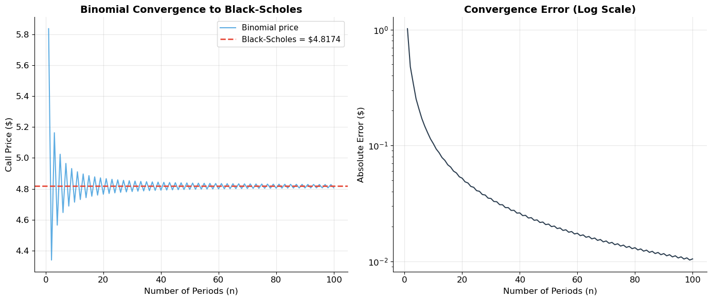

Black-Scholes price: $4.8174
  n =   5: Binomial = $5.0237, error = $0.2063
  n =  10: Binomial = $4.7139, error = $0.1035
  n =  25: Binomial = $4.8582, error = $0.0407
  n =  50: Binomial = $4.7965, error = $0.0209
  n = 100: Binomial = $4.8070, error = $0.0105

As n → ∞, the binomial model converges to Black-Scholes.
In practice, n = 50-100 steps gives excellent accuracy.

7. The Black-Scholes Formula¶

The Continuous-Time Limit¶

As the number of binomial periods $n \to \infty$ (with the period length shrinking proportionally), the binomial model converges to the Black-Scholes-Merton formula:

\boxed{C = S_0 N(d_1) - K e^{-rT} N(d_2)}

(10)

\boxed{P = K e^{-rT} N(-d_2) - S_0 N(-d_1)}

(11)

where:

d_1 = \frac{\ln(S_0/K) + (r + \sigma^2/2)T}{\sigma\sqrt{T}}, \qquad d_2 = d_1 - \sigma\sqrt{T}

(12)

$N(\cdot)$ : cumulative standard normal distribution
$\sigma$ : annualized volatility of the underlying
$r$ : continuously compounded risk-free rate
$T$ : time to expiration (in years)

Interpretation¶

The call price $C = S_0 N(d_1) - Ke^{-rT}N(d_2)$ is the cost of the replicating portfolio:

$N(d_1) = \Delta$ = number of shares (the option’s delta)
$Ke^{-rT}N(d_2)$ = dollars borrowed

Just like the binomial model: a call is a leveraged stock position. The delta $N(d_1)$ is the continuous-time analogue of $\Delta^*$ from the binomial model.

Five Inputs, No Probability¶

The Black-Scholes formula requires only: $S_0$ , $K$ , $T$ , $r$ , and $\sigma$ . Like the binomial model, it does not require the expected return on the stock or investors’ risk preferences.

# ============================================================
# Black-Scholes Pricing and the Greeks
# ============================================================
# ▶ MODIFY AND RE-RUN
S0 = 50
K = 50
T = 30 / 365   # 30 days (matching lecture notes example)
r = np.log(1.05895)  # continuously compounded (~5.73%)
sigma = 0.30
# ============================================================

C = black_scholes_call(S0, K, T, r, sigma)
P = black_scholes_put(S0, K, T, r, sigma)

d1 = (np.log(S0 / K) + (r + sigma**2 / 2) * T) / (sigma * np.sqrt(T))
d2 = d1 - sigma * np.sqrt(T)

print("=" * 65)
print("BLACK-SCHOLES PRICING — Lecture Notes Example")
print("=" * 65)
print(f"S₀ = ${S0}, K = ${K}, T = {T:.4f} yr ({T*365:.0f} days), r = {r:.4f}, σ = {sigma:.0%}")
print(f"\nd₁ = [ln(S/K) + (r + σ²/2)T] / (σ√T)")
print(f"   = [ln({S0}/{K}) + ({r:.4f} + {sigma**2/2:.4f})×{T:.4f}] / ({sigma}×{np.sqrt(T):.4f})")
print(f"   = {d1:.6f}")
print(f"d₂ = d₁ - σ√T = {d1:.6f} - {sigma*np.sqrt(T):.6f} = {d2:.6f}")
print(f"\nN(d₁) = {norm.cdf(d1):.6f}  (delta)")
print(f"N(d₂) = {norm.cdf(d2):.6f}")
print(f"\nCall: C = S·N(d₁) - K·e^(-rT)·N(d₂)")
print(f"       = {S0}×{norm.cdf(d1):.6f} - {K}×{np.exp(-r*T):.6f}×{norm.cdf(d2):.6f}")
print(f"       = ${C:.4f}")
print(f"\nPut:  P = K·e^(-rT)·N(-d₂) - S·N(-d₁)")
print(f"       = ${P:.4f}")

# Verify put-call parity
parity_check = C + K * np.exp(-r * T) - P - S0
print(f"\nPut-call parity check: C + K·e^(-rT) - P - S = {parity_check:.10f} ≈ 0 ✓")

=================================================================
BLACK-SCHOLES PRICING — Lecture Notes Example
=================================================================
S₀ = $50, K = $50, T = 0.0822 yr (30 days), r = 0.0573, σ = 30%

d₁ = [ln(S/K) + (r + σ²/2)T] / (σ√T)
   = [ln(50/50) + (0.0573 + 0.0450)×0.0822] / (0.3×0.2867)
   = 0.097740
d₂ = d₁ - σ√T = 0.097740 - 0.086007 = 0.011733

N(d₁) = 0.538931  (delta)
N(d₂) = 0.504681

Call: C = S·N(d₁) - K·e^(-rT)·N(d₂)
       = 50×0.538931 - 50×0.995303×0.504681
       = $1.8310

Put:  P = K·e^(-rT)·N(-d₂) - S·N(-d₁)
       = $1.5962

Put-call parity check: C + K·e^(-rT) - P - S = 0.0000000000 ≈ 0 ✓

# ============================================================
# Sensitivity Analysis: The Greeks (Visually)
# ============================================================
S0 = 50; K = 50; T = 0.25; r = 0.05; sigma = 0.30

fig, axes = plt.subplots(2, 3, figsize=(18, 10))

# 1. Price vs. S (delta)
S_range = np.linspace(30, 70, 200)
calls = [black_scholes_call(S, K, T, r, sigma) for S in S_range]
puts = [black_scholes_put(S, K, T, r, sigma) for S in S_range]
intrinsic_call = [max(S - K, 0) for S in S_range]
intrinsic_put = [max(K - S, 0) for S in S_range]

axes[0, 0].plot(S_range, calls, color='#3498db', linewidth=3, label='Call')
axes[0, 0].plot(S_range, intrinsic_call, color='#3498db', linewidth=1.5, linestyle=':', label='Intrinsic')
axes[0, 0].plot(S_range, puts, color='#e74c3c', linewidth=3, label='Put')
axes[0, 0].plot(S_range, intrinsic_put, color='#e74c3c', linewidth=1.5, linestyle=':', label='Intrinsic')
axes[0, 0].set_xlabel('Stock Price ($)', fontsize=11)
axes[0, 0].set_ylabel('Option Price ($)', fontsize=11)
axes[0, 0].set_title('Price vs. Stock Price', fontsize=13, fontweight='bold')
axes[0, 0].legend(fontsize=9)
axes[0, 0].axvline(x=K, color='gray', linewidth=1, linestyle=':', alpha=0.4)

# 2. Price vs. sigma (vega)
sig_range = np.linspace(0.05, 0.60, 200)
c_sig = [black_scholes_call(S0, K, T, r, s) for s in sig_range]
p_sig = [black_scholes_put(S0, K, T, r, s) for s in sig_range]
axes[0, 1].plot(sig_range * 100, c_sig, color='#3498db', linewidth=3, label='Call')
axes[0, 1].plot(sig_range * 100, p_sig, color='#e74c3c', linewidth=3, label='Put')
axes[0, 1].set_xlabel('Volatility σ (%)', fontsize=11)
axes[0, 1].set_ylabel('Option Price ($)', fontsize=11)
axes[0, 1].set_title('Price vs. Volatility (Vega)', fontsize=13, fontweight='bold')
axes[0, 1].legend(fontsize=10)

# 3. Price vs. T (theta)
T_range = np.linspace(0.01, 1.0, 200)
c_T = [black_scholes_call(S0, K, t, r, sigma) for t in T_range]
p_T = [black_scholes_put(S0, K, t, r, sigma) for t in T_range]
axes[0, 2].plot(T_range * 365, c_T, color='#3498db', linewidth=3, label='Call')
axes[0, 2].plot(T_range * 365, p_T, color='#e74c3c', linewidth=3, label='Put')
axes[0, 2].set_xlabel('Days to Expiration', fontsize=11)
axes[0, 2].set_ylabel('Option Price ($)', fontsize=11)
axes[0, 2].set_title('Price vs. Time (Theta)', fontsize=13, fontweight='bold')
axes[0, 2].legend(fontsize=10)
axes[0, 2].annotate('Time decay\naccelerates', xy=(60, c_T[int(60/365*200)]),
                    xytext=(150, c_T[int(60/365*200)] + 1), fontsize=9, color='#2c3e50',
                    arrowprops=dict(arrowstyle='->', color='#2c3e50'))

# 4. Delta vs. S
deltas_call = [norm.cdf((np.log(S/K) + (r + sigma**2/2)*T) / (sigma*np.sqrt(T))) for S in S_range]
deltas_put = [norm.cdf((np.log(S/K) + (r + sigma**2/2)*T) / (sigma*np.sqrt(T))) - 1 for S in S_range]
axes[1, 0].plot(S_range, deltas_call, color='#3498db', linewidth=3, label='Call Δ')
axes[1, 0].plot(S_range, deltas_put, color='#e74c3c', linewidth=3, label='Put Δ')
axes[1, 0].axhline(y=0, color='gray', linewidth=1, alpha=0.3)
axes[1, 0].axhline(y=0.5, color='gray', linewidth=1, linestyle=':', alpha=0.3)
axes[1, 0].axvline(x=K, color='gray', linewidth=1, linestyle=':', alpha=0.4)
axes[1, 0].set_xlabel('Stock Price ($)', fontsize=11)
axes[1, 0].set_ylabel('Delta (Δ)', fontsize=11)
axes[1, 0].set_title('Delta vs. Stock Price', fontsize=13, fontweight='bold')
axes[1, 0].legend(fontsize=10)

# 5. Delta vs. T (for ATM)
T_range2 = np.linspace(0.01, 1.0, 200)
deltas_time = [norm.cdf((np.log(S0/K) + (r + sigma**2/2)*t) / (sigma*np.sqrt(t))) for t in T_range2]
axes[1, 1].plot(T_range2 * 365, deltas_time, color='#2c3e50', linewidth=3)
axes[1, 1].set_xlabel('Days to Expiration', fontsize=11)
axes[1, 1].set_ylabel('Call Delta (Δ)', fontsize=11)
axes[1, 1].set_title('ATM Call Delta vs. Time', fontsize=13, fontweight='bold')
axes[1, 1].axhline(y=0.5, color='gray', linewidth=1, linestyle=':', alpha=0.5)

# 6. Price vs. r (rho)
r_range = np.linspace(0.001, 0.15, 200)
c_r = [black_scholes_call(S0, K, T, rr, sigma) for rr in r_range]
p_r = [black_scholes_put(S0, K, T, rr, sigma) for rr in r_range]
axes[1, 2].plot(r_range * 100, c_r, color='#3498db', linewidth=3, label='Call')
axes[1, 2].plot(r_range * 100, p_r, color='#e74c3c', linewidth=3, label='Put')
axes[1, 2].set_xlabel('Risk-free Rate r (%)', fontsize=11)
axes[1, 2].set_ylabel('Option Price ($)', fontsize=11)
axes[1, 2].set_title('Price vs. Interest Rate (Rho)', fontsize=13, fontweight='bold')
axes[1, 2].legend(fontsize=10)

plt.tight_layout()
plt.show()

print("Key sensitivity insights:")
print("• Stock price: Call Δ ∈ [0,1]; deep ITM → Δ≈1; deep OTM → Δ≈0; ATM → Δ≈0.5")
print("• Volatility: BOTH calls and puts increase with σ (unique to options)")
print("• Time: Options lose value as expiration approaches ('time decay' / 'theta')")
print("• Time decay accelerates near expiration — the last 30 days are critical")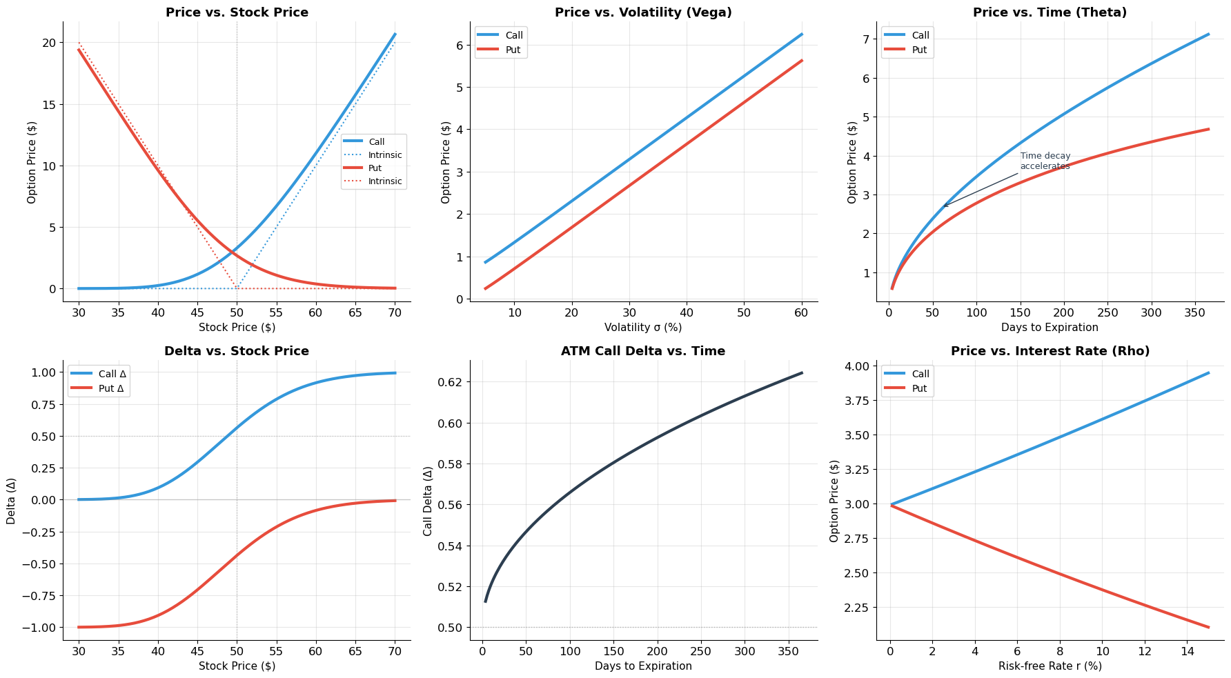

Key sensitivity insights:
• Stock price: Call Δ ∈ [0,1]; deep ITM → Δ≈1; deep OTM → Δ≈0; ATM → Δ≈0.5
• Volatility: BOTH calls and puts increase with σ (unique to options)
• Time: Options lose value as expiration approaches ('time decay' / 'theta')
• Time decay accelerates near expiration — the last 30 days are critical

8. A Brief History of Option-Pricing Theory¶

Lo devotes several slides (22–27) to the intellectual history of option pricing — a story he clearly loves telling. Here is the abbreviated timeline:

The Pioneers¶

Year	Scholar	Contribution
c.1565	Cardano	Liber De Ludo Aleae: first mathematical treatment of fair games; precursor to the random walk
1900	Bachelier	Théorie de la Spéculation: first mathematical model of Brownian motion; modeled warrant prices on the Paris Bourse. Anticipated much of modern finance by 50+ years
1956	Kruizenga	MIT PhD thesis (Samuelson adviser): empirical study of puts and calls
1961	Sprenkle	Yale PhD thesis (Tobin adviser): warrant pricing using expected payoffs
1965	Samuelson	“Rational Theory of Warrant Pricing” — correct expected value calculation but still required risk preferences
1969	Samuelson & Merton	“A Complete Model of Warrant Pricing that Maximizes Utility” — first to bring utility theory to bear

The Breakthrough¶

Year	Scholar	Contribution
1973	Black & Scholes	“The Pricing of Options and Corporate Liabilities” — derived the pricing formula by eliminating market risk via CAPM
1973	Merton	“Rational Theory of Option Pricing” — independent derivation using continuous-time dynamic hedging; more general and elegant
1979	Cox, Ross & Rubinstein	Binomial option-pricing model — made the idea accessible and computationally tractable

Why It Matters¶

Lo emphasizes Merton’s contribution: the ability to replicate any derivative by dynamic trading is not just a pricing formula — it’s a “production process” for derivatives. This insight spawned three entire industries: listed options, OTC structured products, and credit derivatives.

9. Exercises¶

Exercise 1: Payoff Diagrams and Strategies¶

(a) Draw the payoff diagram for a butterfly spread: buy a call at $K_1 = 45$ , sell two calls at $K_2 = 50$ , buy a call at $K_3 = 55$ . What view of the market does this strategy express?

(b) Construct a bear put spread (buy put at $K_2 = 55$ , sell put at $K_1 = 45$ ). Compare the profit profile with a naked long put at $K = 55$ .

(c) You believe a stock currently at $50 will move dramatically in the next month but you’re unsure of the direction. A 1-month ATM call costs $3 and a 1-month ATM put costs $2.50. Construct a straddle and determine the breakeven stock prices.

(d) Using put-call parity, if $S_0 = \$50$ , $K = \$50$ , $r = 5\%$ , $T = 0.5$ years, and $C = \$5.00$ , what must the put price be? If the market put trades at $4.00, describe the arbitrage.

# Exercise 1 — Workspace
# (a) Butterfly spread
# K1, K2, K3 = 45, 50, 55
# S = np.linspace(35, 65, 200)
# payoff = np.maximum(S-K1,0) - 2*np.maximum(S-K2,0) + np.maximum(S-K3,0)
# plt.plot(S, payoff); plt.show()
# A butterfly bets that the stock stays NEAR K2 — a low-volatility bet
#
# (d) P = C + K*exp(-rT) - S
# P_theoretical = 5 + 50*np.exp(-0.05*0.5) - 50
# If market P = 4.00 < theoretical:
#   Buy put, sell call, buy stock, borrow K*exp(-rT)
#   Profit = P_theoretical - 4.00

Exercise 2: Binomial Option Pricing¶

A stock is currently at $100. Each period, it can go up by 20% ( $u = 1.20$ ) or down by 10% ( $d = 0.90$ ). The risk-free rate is 5% per period (gross $r = 1.05$ ). Consider a European call with strike $K = 100$ .

(a) Build the one-period binomial tree. Compute the replicating portfolio ( $\Delta^*$ , $B^*$ ) and the call price.

(b) Extend to two periods. Show the complete stock tree and option tree. Verify by backward induction.

(c) Compute the risk-neutral probability $q$ . Verify the option price using the risk-neutral pricing formula: $C_0 = \frac{1}{r^2}[q^2 C_{uu} + 2q(1-q)C_{ud} + (1-q)^2 C_{dd}]$ .

(d) Now price a European put with the same parameters. Verify that put-call parity holds in the binomial model.

# Exercise 2 — Workspace
# S0, K, u, d, r = 100, 100, 1.20, 0.90, 1.05
#
# (a) One period:
# C0, delta, B, Cu, Cd, q = binomial_one_period(S0, K, u, d, r)
#
# (b) Two periods:
# C0_2, stock, opt, delta_tree = binomial_tree(S0, K, u, d, r, 2, 'call')
# draw_binomial_tree(stock, opt, delta_tree, 2, 'Exercise 2', K)
#
# (c) Risk-neutral: q = (r-d)/(u-d)
# C0_rn = (q**2 * opt[0,2] + 2*q*(1-q)*opt[1,2] + (1-q)**2*opt[2,2]) / r**2
#
# (d) Put:
# P0, stock_p, opt_p, delta_p = binomial_tree(S0, K, u, d, r, 2, 'put')
# Parity check: C0_2 + K/r**2 should equal P0 + S0

Exercise 3: Black-Scholes and Applications¶

A non-dividend-paying stock trades at $100 with volatility $\sigma = 25\%$ . The risk-free rate is 3%.

(a) Price a 3-month European call with strike $105. Price the corresponding put.

(b) The market quotes the 3-month ATM (K=100) call at $5.50. What implied volatility does this correspond to? (Use numerical root-finding.)

(c) Compute the delta of the call from part (a). If you sell 100 call contracts (each covering 100 shares), how many shares must you buy to be delta-neutral?

(d) A portfolio manager holds 10,000 shares of the stock. She wants to create a protective put using Black-Scholes delta hedging instead of buying actual puts. How many shares should she sell to replicate the protective put payoff? How does this “portfolio insurance” strategy work in practice?

# Exercise 3 — Workspace
# S0, sigma, r = 100, 0.25, 0.03
#
# (a) T = 0.25; K = 105
# C = black_scholes_call(S0, 105, 0.25, 0.03, 0.25)
# P = black_scholes_put(S0, 105, 0.25, 0.03, 0.25)
#
# (b) Implied volatility
# target = 5.50; K_atm = 100
# iv = brentq(lambda s: black_scholes_call(100, 100, 0.25, 0.03, s) - 5.50, 0.01, 1.0)
# print(f"Implied vol = {iv:.2%}")
#
# (c) Delta
# d1 = (np.log(S0/105) + (0.03 + 0.25**2/2)*0.25) / (0.25*np.sqrt(0.25))
# delta = norm.cdf(d1)
# shares_to_buy = delta * 100 * 100  # 100 contracts × 100 shares
#
# (d) Protective put delta = 1 + delta_put = 1 - (1 - delta_call) = delta_call
# shares_to_hold = delta_call * 10000

Key Takeaways — Session 8¶

Options give the right, not the obligation to buy (call) or sell (put) at a fixed price. This creates nonlinear payoffs — fundamentally different from forwards/futures.
Payoff diagrams are the visual language of options. Long calls have unlimited upside and limited downside; long puts have limited upside and limited downside. Short positions reverse these profiles.
Option strategies combine positions to create customized payoff profiles: protective puts (insurance), spreads (directional bets), straddles (volatility bets), and many more.
Put-call parity ( $C + KB = P + S$ ) is a model-free no-arbitrage relation. It links calls, puts, stocks, and bonds. Violations create riskless profit opportunities.
Volatility increases option value — unique among securities. Higher uncertainty means higher expected payoff due to the option’s asymmetric nature.
The binomial model prices options by replication: construct a portfolio of stocks and bonds that matches the option payoff, then invoke no-arbitrage. The probability $p$ drops out — only $S$ , $K$ , $u$ , $d$ , and $r$ matter.
Black-Scholes is the continuous-time limit of the binomial model: $C = SN(d_1) - Ke^{-rT}N(d_2)$ . Five inputs, no probability, no risk preferences. A call is equivalent to a leveraged stock position ( $\Delta$ shares financed by borrowing).
Historical significance: Option pricing theory (Bachelier → Black-Scholes-Merton → Cox-Ross-Rubinstein) is one of the great intellectual achievements of 20th-century economics, creating the theoretical foundation for the entire derivatives industry.

References¶

Brealey, R.A., Myers, S.C., and Allen, F. Principles of Corporate Finance, Chapters 20–21.
MIT OCW 15.401: Options
Black, F. and Scholes, M. (1973). “The Pricing of Options and Corporate Liabilities.” Journal of Political Economy, 81, 637–659.
Merton, R. (1973). “Theory of Rational Option Pricing.” Bell Journal of Economics and Management Science, 4, 141–183.
Cox, J., Ross, S., and Rubinstein, M. (1979). “Option Pricing: A Simplified Approach.” Journal of Financial Economics, 7, 229–263.
Bachelier, L. (1900). “Théorie de la Spéculation.” Annales de l’École Normale Supérieure, 3.

Next: Session 9 — Risk and Return — measuring risk, diversification, systematic vs. idiosyncratic risk, and the introduction to portfolio theory.